library(tidyverse)
library(knitr)
library(tidymodels)
library(pROC)
library(Stat2Data)AE 06: Exam 02 review
Important
There is no repo for this AE.
Exercise 1
Suppose you fit a simple linear regression model.
Draw a scatterplot that contains an observation with large leverage but low Cook’s distance.
Draw a scatterplot that contains an observation with large leverage and high Cook’s distance.
Draw a scatterplot that contains an observation with a large standardized residual.
Exercise 2
Describe what it means for \(\hat{\boldsymbol{\beta}}\) to be the maximum likelihood estimator.
What are properties of MLEs?
Exercise 3
This exercise is adapted from Casella and Berger (2024).
Suppose there are \(n\) observations \((x_1, y_1), \ldots, (x_n, y_n)\), such that the relationship between \(X\) and \(Y\) can be summarized as \[ y_i = \beta x_i^2 + \epsilon_i \hspace{8mm} \epsilon_i \sim N(0,\sigma^2_{\epsilon}) \]
Find the maximum likelihood estimator of \(\beta\) .
Is the MLE unbiased?
Note
Use this data analysis scenario for Exercises 4 - 6.
The data for this analysis is about credit card customers. It can be found in the file credit.csv. The following variables are in the data set:
income: Income in $1,000’slimit: Credit limitrating: Credit ratingcards: Number of credit cardsage: Age in yearseducation: Number of years of educationown: Whether an individual owns their home (NoorYes)student: Whether the individual was a student (NoorYes)married: Whether the individual was married (NoandYes)region: Region the individual is from (South,East, andWest)balance: Average credit card balance in $.
credit <- read_csv("data/credit.csv") |>
  mutate(maxed = factor(if_else(balance == 0, 1, 0)))
The objective of this analysis is to predict whether a person has maxed out their credit card, i.e., had $0 average card balance.
We’ll start with a model predicting the odds of maxed = 1 using income, rating, and region.
credit_fit <- glm(maxed ~ income + rating + region, data = credit,
                  family = "binomial")

tidy(credit_fit) |>
kable(digits = 3)| term | estimate | std.error | statistic | p.value |
|---|---|---|---|---|
| (Intercept) | 9.898 | 1.449 | 6.829 | 0.000 |
| income | 0.113 | 0.021 | 5.273 | 0.000 |
| rating | -0.057 | 0.008 | -7.397 | 0.000 |
| regionSouth | -0.595 | 0.604 | -0.985 | 0.324 |
| regionWest | -0.082 | 0.649 | -0.126 | 0.900 |
Exercise 4
Write the interpretation of
incomein terms of the odds of maxing out a credit card.What is the odds ratio of the South versus the East regions?
Suppose there are two individuals. Individual 1 has an income of $64,000, a credit rating of 590, and is from the South region. Individual 2 has an income of $135,000, a credit rating of 695, and is from the East region. Use the equation above to show how the odds of maxing out a credit card differ between Individual 1 and Individual 2.
Exercise 5
We consider adding the interaction between region and income to the current model. We use a drop-in-deviance test to determine whether or not to add the interaction term. The output for the drop-in-deviance test is below.
credit_fit_int <- glm(maxed ~ income + rating + region + region * income, data = credit,
                  family = "binomial")

anova(credit_fit, credit_fit_int, test = "Chisq") |>
kable(digits = 2)| Resid. Df | Resid. Dev | Df | Deviance | Pr(>Chi) |
|---|---|---|---|---|
| 395 | 107.66 | NA | NA | NA |
| 393 | 106.53 | 2 | 1.13 | 0.57 |
- State the null and alternative hypotheses in words and using mathematical notation.
- Describe what the test statistic \(G\) means in the context of the data.
- Show why the degrees of freedom for the test statistic are equal to 2.
- State the conclusion in the context of the data.
Exercise 6
Use the model credit_fit that includes the main effects for income, rating, and region. The ROC curve and AUC are below.
credit_fit_aug <- augment(credit_fit, type.predict = "response")

credit_fit_aug |>
  roc_curve(
    maxed,
    .fitted,
    event_level = "second"
  ) |>
  autoplot()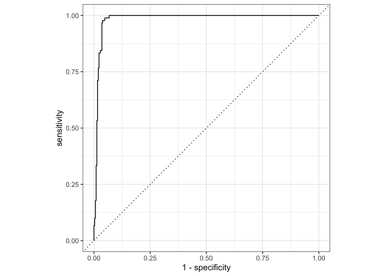
credit_fit_aug |>
  roc_auc(
    maxed,
    .fitted,
    event_level = "second"
  )
# A tibble: 1 × 3
.metric .estimator .estimate
<chr> <chr> <dbl>
1 roc_auc binary 0.983- Based on the AUC, do you think this model sufficiently identifies those who will max out their credit card vs. those who will not? Explain.
- Suppose a credit card company uses your model to inform the credit limit to give to new customers. Do you think they would prioritize having high sensitivity or high specificity? Explain.
- Based on your response to part(b), would you set a high (closer to 1) or low (closer to 0) classification threshold?
References
Casella, George, and Roger Berger. 2024. Statistical Inference. CRC Press.