Multiple linear regression
Types of predictors
January 29, 2026
Announcements
HW 01 due TODAY at 11:59pm
(Optional) Submit team request by TODAY at 5pm: https://forms.office.com/r/3WHjriZjM9
Statistics experience due April 2
SSMU Mini DataFest - February 8
Topics
Categorical predictors
Centering quantitative predictors
Standardizing quantitative predictors
Interaction terms
Computing setup
Data: Peer-to-peer lender
Today’s data is a sample of 50 loans made through a peer-to-peer lending club. The data is in the loan50 data frame in the openintro R package.
# A tibble: 50 × 4
   annual_income_th debt_to_income verified_income interest_rate
              <dbl>          <dbl> <fct>                   <dbl>
 1             59           0.558  Not Verified            10.9
 2             60           1.31   Not Verified             9.92
 3             75           1.06   Verified                26.3
 4             75           0.574  Not Verified             9.92
 5            254           0.238  Not Verified             9.43
 6             67           1.08   Source Verified          9.92
 7             28.8         0.0997 Source Verified         17.1
 8             80           0.351  Not Verified             6.08
 9             34           0.698  Not Verified             7.97
10             80           0.167  Source Verified         12.6
# ℹ 40 more rows
Variables
Predictors:
annual_income_th: Annual income (in $1000s)debt_to_income: Debt-to-income ratio, i.e. the percentage of a borrower’s total debt divided by their total incomeverified_income: Whether borrower’s income source and amount have been verified (Not Verified,Source Verified,Verified)
Response: interest_rate: Interest rate for the loan
Response vs. predictors
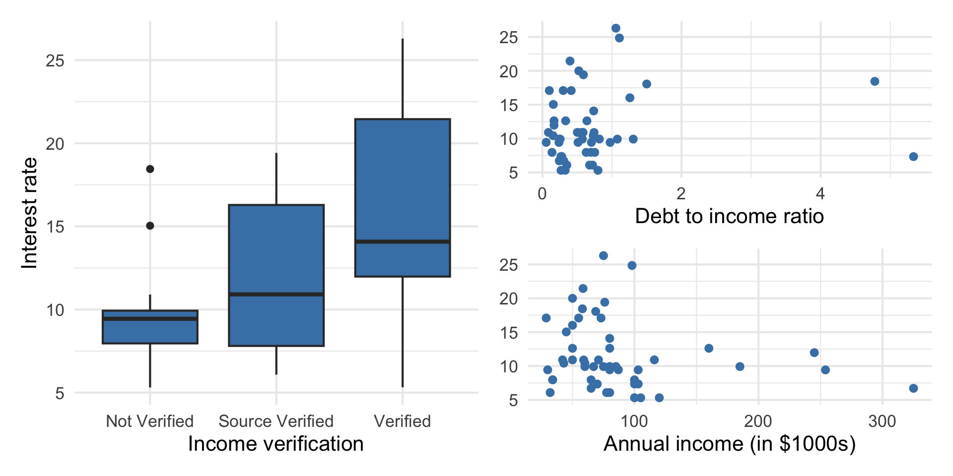
Goal: Use these predictors in a single model to understand variability in interest rate.
Model fit in R
| term | estimate | std.error | statistic | p.value |
|---|---|---|---|---|
| (Intercept) | 10.726 | 1.507 | 7.116 | 0.000 |
| debt_to_income | 0.671 | 0.676 | 0.993 | 0.326 |
| verified_incomeSource Verified | 2.211 | 1.399 | 1.581 | 0.121 |
| verified_incomeVerified | 6.880 | 1.801 | 3.820 | 0.000 |
| annual_income_th | -0.021 | 0.011 | -1.804 | 0.078 |
Categorical predictors
Matrix form of multiple linear regression
\[ \underbrace{ \begin{bmatrix} y_1 \\ \vdots \\ y_n \end{bmatrix} }_ {\mathbf{y}} \hspace{3mm} = \hspace{3mm} \underbrace{ \begin{bmatrix} 1 &x_{11} & \dots & x_{1p}\\ \vdots & \vdots &\ddots & \vdots \\ 1 & x_{n1} & \dots &x_{np} \end{bmatrix} }_{\mathbf{X}} \hspace{2mm} \underbrace{ \begin{bmatrix} \beta_0 \\ \beta_1 \\ \vdots \\ \beta_p \end{bmatrix} }_{\boldsymbol{\beta}} \hspace{3mm} + \hspace{3mm} \underbrace{ \begin{bmatrix} \epsilon_1 \\ \vdots\\ \epsilon_n \end{bmatrix} }_\boldsymbol{\epsilon} \]
Indicator variables
Suppose there is a categorical variable with \(k\) levels
We can make \(k\) indicator variables from the data - one indicator for each level
An indicator (dummy) variable takes values 1 or 0
1 if the observation belongs to that level
0 if the observation does not belong to that level
Indicator variables
Suppose we want to predict the amount of sleep a Duke student gets based on whether they are in Pratt (Pratt Yes/ No are the only two options). Consider the model
\[ Sleep_i = \beta_0 + \beta_1\mathbf{1}(Pratt_i = \texttt{Yes}) + \beta_2\mathbf{1}(Pratt_i = \texttt{No}) \]
Write out the design matrix for this hypothesized linear model.
Demonstrate that the design matrix is not of full column rank (that is, affirmatively provide one of the columns in terms of the others).
Use this intuition to explain why when we include categorical predictors, we cannot include both indicators for every level of the variable and an intercept.
Indicator variables for verified_income
# A tibble: 3 × 4
  verified_income not_verified source_verified verified
  <fct>           <fct>        <fct>           <fct>
1 Not Verified    1            0               0
2 Verified        0            0               1
3 Source Verified 0            1               0
Trying to use all indicators in R
Run the code below to fit a model using debt_to_income, annual_income_th, and all the indicator variables for verified_income to predict interest_rate. What do you notice about the model output? Why did this happen?
Indicator variables in the model
Given a categorical predictor with \(k\) levels…
- Use \(k-1\) indicator variables in the model
- The baseline is the category that doesn’t have a term in the model
- This is also called the reference level
- The coefficients of the indicator variables in the model are interpreted as the expected change in the response compared to the baseline, holding all other variables constant.
AE: Model in R
Now let’s take a look at the design matrix for the model with predictors debt_to_income, annual_income_th, and verified_income.
How does R choose the baseline level by default?
Exploring indicator variables
| term | estimate | std.error | statistic | p.value | conf.low | conf.high |
|---|---|---|---|---|---|---|
| (Intercept) | 10.726 | 1.507 | 7.116 | 0.000 | 7.690 | 13.762 |
| debt_to_income | 0.671 | 0.676 | 0.993 | 0.326 | -0.690 | 2.033 |
| verified_incomeSource Verified | 2.211 | 1.399 | 1.581 | 0.121 | -0.606 | 5.028 |
| verified_incomeVerified | 6.880 | 1.801 | 3.820 | 0.000 | 3.253 | 10.508 |
| annual_income_th | -0.021 | 0.011 | -1.804 | 0.078 | -0.043 | 0.002 |
What is the intercept for individuals with
Not verified income?
Source verified income?
Verified income?
Interpreting verified_income
| term | estimate | std.error | statistic | p.value | conf.low | conf.high |
|---|---|---|---|---|---|---|
| (Intercept) | 10.726 | 1.507 | 7.116 | 0.000 | 7.690 | 13.762 |
| debt_to_income | 0.671 | 0.676 | 0.993 | 0.326 | -0.690 | 2.033 |
| verified_incomeSource Verified | 2.211 | 1.399 | 1.581 | 0.121 | -0.606 | 5.028 |
| verified_incomeVerified | 6.880 | 1.801 | 3.820 | 0.000 | 3.253 | 10.508 |
| annual_income_th | -0.021 | 0.011 | -1.804 | 0.078 | -0.043 | 0.002 |
- The baseline level is
Not verified. - People with source verified income are expected to take a loan with an interest rate that is 2.211% higher, on average, than the rate on loans to those whose income is not verified, holding all else constant.
Centering
Centering a quantitative predictor means shifting every value by some constant \(C\)
One common type of centering is mean-centering, in which every value of a predictor is shifted by its mean
Only quantitative predictors are centered
Center all quantitative predictors in the model for ease of interpretation
What is one reason we might want to center the quantitative predictors? What are the units of centered variables?
Centering
Use the scale() function with center = TRUE and scale = FALSE to mean-center variables
| term | estimate | std.error | statistic | p.value |
|---|---|---|---|---|
| (Intercept) | 9.444 | 0.977 | 9.663 | 0.000 |
| debt_to_inc_cent | 0.671 | 0.676 | 0.993 | 0.326 |
| verified_incomeSource Verified | 2.211 | 1.399 | 1.581 | 0.121 |
| verified_incomeVerified | 6.880 | 1.801 | 3.820 | 0.000 |
| annual_inc_cent | -0.021 | 0.011 | -1.804 | 0.078 |
Centering
| Term | Original Model | Centered Model |
|---|---|---|
| (Intercept) | 10.726 | 9.444 |
| debt_to_income | 0.671 | 0.671 |
| verified_incomeSource Verified | 2.211 | 2.211 |
| verified_incomeVerified | 6.880 | 6.880 |
| annual_income_th | -0.021 | -0.021 |
How has the model changed? How has the model remained the same?
Standardizing
Standardizing a quantitative predictor mean shifting every value by the mean and dividing by the standard deviation of that variable
Only quantitative predictors are standardized
Standardize all quantitative predictors in the model for ease of interpretation
What is one reason we might want to standardize the quantitative predictors? What are the units of standardized variables?
Standardizing
Use the scale() function with center = TRUE and scale = TRUE to standardized variables
| term | estimate | std.error | statistic | p.value |
|---|---|---|---|---|
| (Intercept) | 9.444 | 0.977 | 9.663 | 0.000 |
| debt_to_inc_std | 0.643 | 0.648 | 0.993 | 0.326 |
| verified_incomeSource Verified | 2.211 | 1.399 | 1.581 | 0.121 |
| verified_incomeVerified | 6.880 | 1.801 | 3.820 | 0.000 |
| annual_inc_std | -1.180 | 0.654 | -1.804 | 0.078 |
Standardizing
| Term | Original Model | Standardized Model |
|---|---|---|
| (Intercept) | 10.726 | 9.444 |
| debt_to_income | 0.671 | 0.643 |
| verified_incomeSource Verified | 2.211 | 2.211 |
| verified_incomeVerified | 6.880 | 6.880 |
| annual_income_th | -0.021 | -1.180 |
How has the model changed? How has the model remained the same?
Interaction terms
Interaction terms
- Sometimes the relationship between a predictor variable and the response depends on the value of another predictor variable.
- This is an interaction effect.
- To account for this, we can include interaction terms in the model.
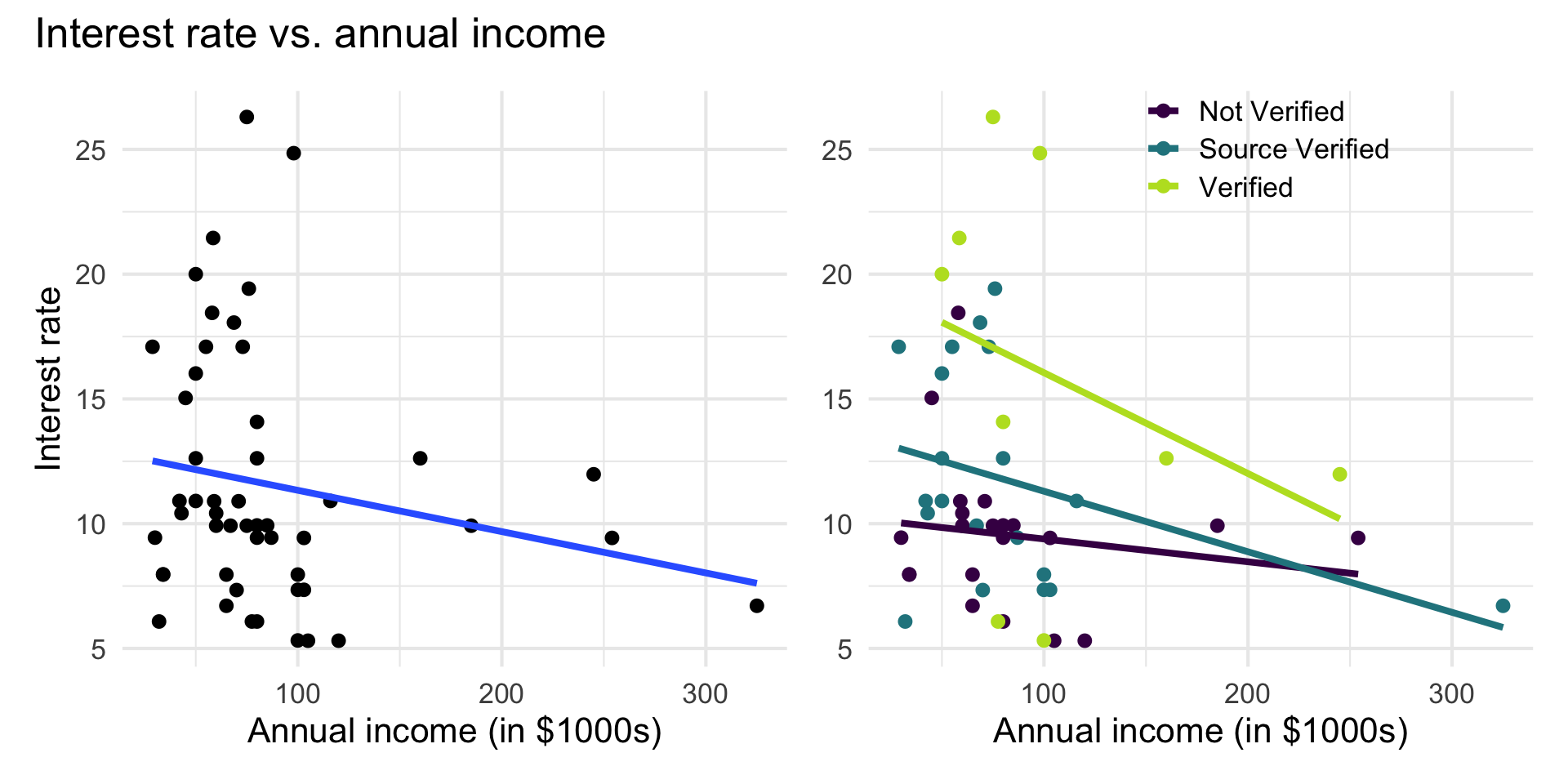
Interest rate vs. annual income
The lines are not parallel indicating there is a potential interaction effect. The slope of annual income differs based on the income verification.
AE: Model with interaction effect
Fit the model with the predictors debt_to_income, annual_income_th, verified_income , and the interaction between annual_income_th and verified_income.
Write the estimated regression equation for the people with
Not Verifiedincome.Write the estimated regression equation for people with
Verifiedincome.
Interaction term in model
| term | estimate | std.error | statistic | p.value |
|---|---|---|---|---|
| (Intercept) | 9.560 | 2.034 | 4.700 | 0.000 |
| debt_to_income | 0.691 | 0.685 | 1.009 | 0.319 |
| verified_incomeSource Verified | 3.577 | 2.539 | 1.409 | 0.166 |
| verified_incomeVerified | 9.923 | 3.654 | 2.716 | 0.009 |
| annual_income_th | -0.007 | 0.020 | -0.341 | 0.735 |
| verified_incomeSource Verified:annual_income_th | -0.016 | 0.026 | -0.643 | 0.523 |
| verified_incomeVerified:annual_income_th | -0.032 | 0.033 | -0.979 | 0.333 |
Interpreting interaction terms
- What the interaction means: The effect of annual income on the interest rate differs by -0.016 when the income is source verified compared to when it is not verified, holding all else constant.
- Interpreting
annual_incomefor source verified: If the income is source verified, we expect the interest rate to decrease by 0.023% (-0.007 + -0.016) for each additional thousand dollars in annual income, holding all else constant.
Indicators and interactions
In general, how do
indicators for categorical predictors impact the model equation?
interaction terms impact the model equation?
Recap
Interpreted categorical predictors
Explored why the model includes \(k-1\) terms for a categorical predictor with \(k\) levels
Fit and interpreted models with centered and standardized variables
Interpreted interaction terms
Next class
- Inference for regression
- Complete Lecture 07 prepare