Inference for regression
Distribution of coefficients
February 05, 2026
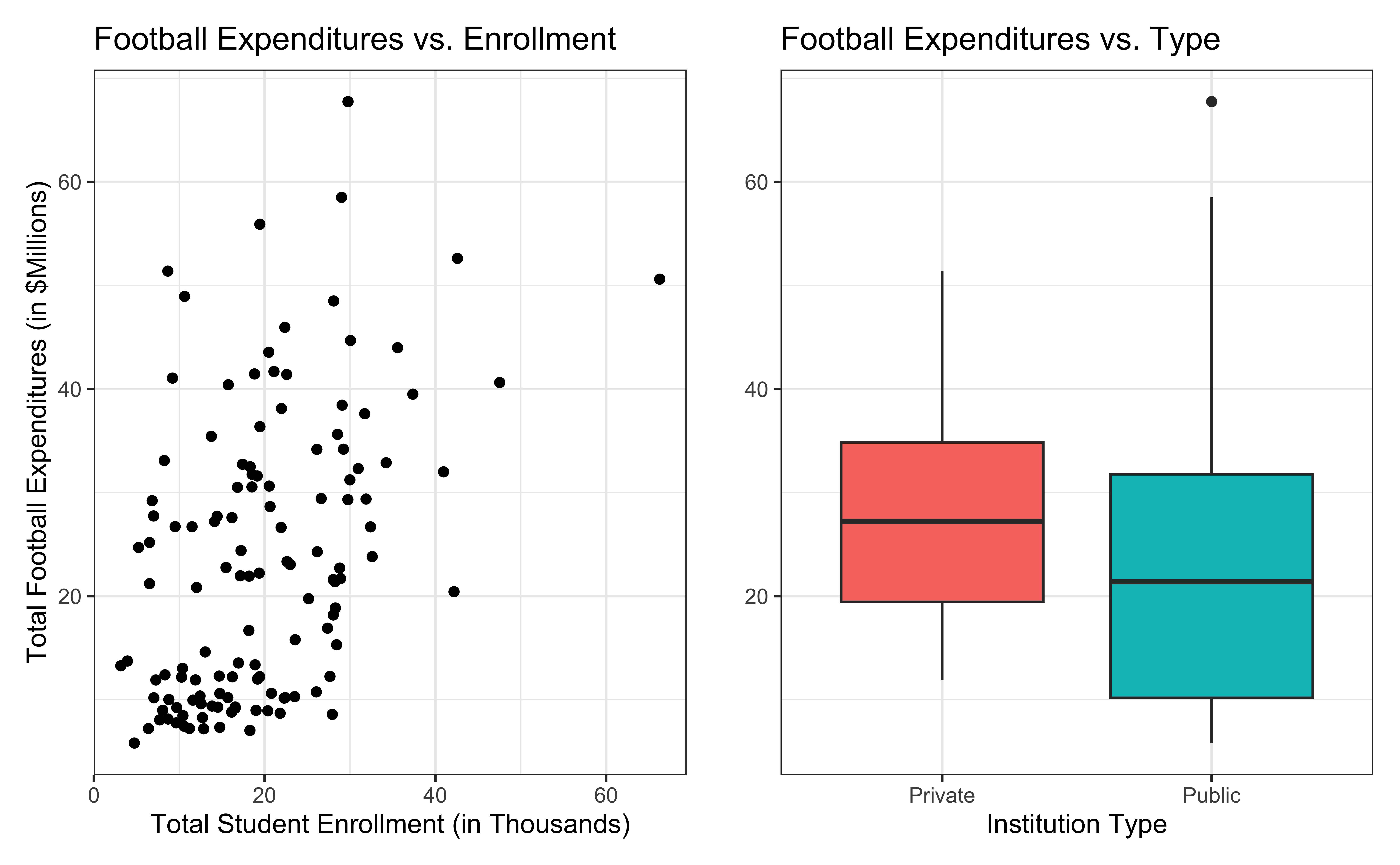
Bivariate EDA
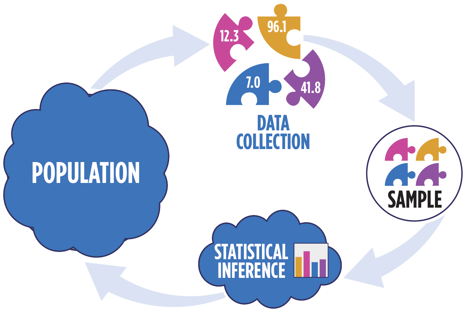
Statistical inference
Statistical inference provides methods and tools so we can use the single observed sample to make valid statements (inferences) about the population it comes from
For our inferences to be valid, the sample should be representative (ideally random) of the population we’re interested in
Visualizing distribution of \(\mathbf{y}|\mathbf{X}\)
\[ \mathbf{y}|\mathbf{X} \sim N(\mathbf{X}\boldsymbol{\beta}, \sigma_\epsilon^2\mathbf{I}) \]
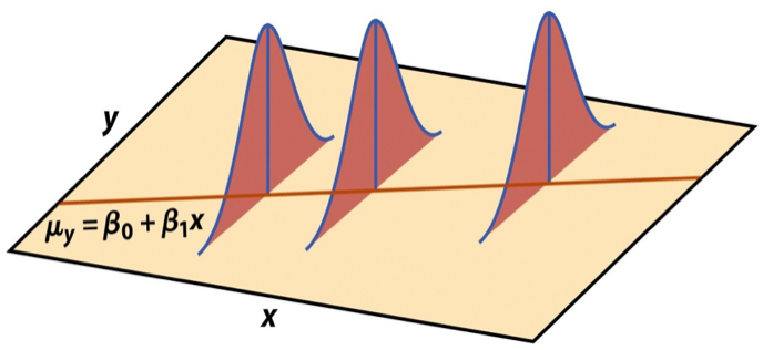
Image source: Introduction to the Practice of Statistics (5th ed)
Last time we showed \(E(\mathbf{y}|\mathbf{X}) = \mathbf{X}\boldsymbol{\beta}\) and \(Var(\mathbf{y}|\mathbf{X}) = \sigma^2_{\epsilon}\mathbf{I}\)
Assumptions for regression
\[ \mathbf{y}|\mathbf{X} \sim N(\mathbf{X}\boldsymbol{\beta}, \sigma_\epsilon^2\mathbf{I}) \]
- Linearity: There is a linear relationship between the response and predictor variables.
- Equal variance: The variability about the least squares line is equal for all combinations of predictors.
- Normality: The distribution of the residuals is normal.
- Independence: The residuals are independent from one another.
Note
We will assume these hold for now and show how to check the assumptions after Exam 01.