Inference for regression

Hypothesis tests + confidence intervals

Prof. Maria Tackett

Feb 10, 2026

Announcements

• Research topics due TODAY at 11:59pm on GitHub

• HW 02 due Thursday, February 12 at 11:59pm

Exam 01 resources

• Exam 01 practice
• Math rules (will be provided on exam)
• Lecture recordings
• Prepare readings (see course schedule)
• Lecture notes
• AEs
• Lab and HW assignments

Topics

• Hypothesis tests for a coefficient \(\beta_j\)

• Confidence intervals for a coefficient \(\beta_j\)

Computing setup

# load packages
library(tidyverse)  
library(tidymodels)  
library(knitr)       
library(kableExtra)  
library(patchwork)   

# set default theme in ggplot2
ggplot2::theme_set(ggplot2::theme_bw())

Data: NCAA Football expenditures

Today’s data come from Equity in Athletics Data Analysis and includes information about sports expenditures and revenues for colleges and universities in the United States. This data set was featured in a March 2022 Tidy Tuesday.

We will focus on the 2019 - 2020 season expenditures on football for institutions in the NCAA - Division 1 FBS. The variables are :

• total_exp_m: Total expenditures on football in the 2019 - 2020 academic year (in millions USD)

• enrollment_th: Total student enrollment in the 2019 - 2020 academic year (in thousands)

• type: institution type (Public or Private)

football <- read_csv("data/ncaa-football-exp.csv")

Regression model

exp_fit <- lm(total_exp_m ~ enrollment_th + type, data = football)
tidy(exp_fit) |>
  kable(digits = 3)

term	estimate	std.error	statistic	p.value
(Intercept)	19.332	2.984	6.478	0
enrollment_th	0.780	0.110	7.074	0
typePublic	-13.226	3.153	-4.195	0

Linear regression model

\[\begin{aligned} \mathbf{Y} = \mathbf{X}\boldsymbol{\beta} + \boldsymbol{\epsilon}, \hspace{8mm} \boldsymbol{\epsilon} \sim N(\mathbf{0}, \sigma^2_{\epsilon}\mathbf{I}) \end{aligned} \]

such that the errors are independent and normally distributed.

• Independent: Knowing the error term for one observation doesn’t tell us about the error term for another observation
• Normally distributed: The distribution follows a particular mathematical model that is unimodal and symmetric
  • \(E(\boldsymbol{\epsilon}) = \mathbf{0}\)
  • \(Var(\boldsymbol{\epsilon}) = \sigma^2_{\epsilon}\mathbf{I}\)

Assumptions for regression

\[ \mathbf{y}|\mathbf{X} \sim N(\mathbf{X}\boldsymbol{\beta}, \sigma_\epsilon^2\mathbf{I}) \]

Image source: Introduction to the Practice of Statistics (5th ed)

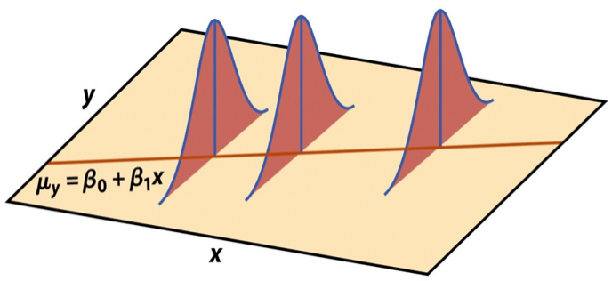
1. Linearity: There is a linear relationship between the response and predictor variables.
2. Constant Variance: The variability about the least squares line is generally constant.
3. Normality: The distribution of the residuals is approximately normal.
4. Independence: The residuals are independent from one another.

Estimating \(\sigma^2_{\epsilon}\)

• Once we fit the model, we can use the residuals to estimate \(\sigma_{\epsilon}^2\)

• The estimated value \(\hat{\sigma}^2_{\epsilon}\) is needed for hypothesis testing and constructing confidence intervals for regression

\[ \hat{\sigma}^2_\epsilon = \frac{SSR}{n - p - 1} = \frac{\mathbf{e}^\mathsf{T}\mathbf{e}}{n-p-1} \]

• The regression standard error \(\hat{\sigma}_{\epsilon}\) is a measure of the average distance between the observations and regression line

\[ \hat{\sigma}_\epsilon = \sqrt{\frac{SSR}{n - p - 1}} = \sqrt{\frac{\mathbf{e}^\mathsf{T}\mathbf{e}}{n - p - 1}} \]

Sampling distribution of \(\hat{\beta}\)

• A sampling distribution is the probability distribution of a statistic for a large number of random samples of size \(n\) from a population

• The sampling distribution of \(\hat{\boldsymbol{\beta}}\) is the probability distribution of the estimated coefficients if we repeatedly took samples of size \(n\) and fit the regression model

\[ \hat{\boldsymbol{\beta}} \sim N(\boldsymbol{\beta}, \sigma^2_\epsilon(\mathbf{X}^\mathsf{T}\mathbf{X})^{-1}) \]

The estimated coefficients \(\hat{\boldsymbol{\beta}}\) are normally distributed with

\[ E(\hat{\boldsymbol{\beta}}) = \boldsymbol{\beta} \hspace{10mm} Var(\hat{\boldsymbol{\beta}}) = \sigma^2_{\epsilon}(\boldsymbol{X}^\mathsf{T}\boldsymbol{X})^{-1} \]

Sampling distribution of \(\hat{\beta}_j\)

\[ \hat{\boldsymbol{\beta}} \sim N(\boldsymbol{\beta}, \sigma^2_\epsilon(\mathbf{X}^\mathsf{T}\mathbf{X})^{-1}) \]

Let \(\mathbf{C} = (\mathbf{X}^\mathsf{T}\mathbf{X})^{-1}\). Then, for each coefficient \(\hat{\beta}_j\),

• \(E(\hat{\beta}_j) = \boldsymbol{\beta}_j\), the \(j^{th}\) element of \(\boldsymbol{\beta}\)

• \(Var(\hat{\beta}_j) = \sigma^2_{\epsilon}C_{jj}\)

• \(Cov(\hat{\beta}_i, \hat{\beta}_j) = \sigma^2_{\epsilon}C_{ij}\)

\(Var(\hat{\boldsymbol{\beta}})\) for NCAA data

X <- model.matrix(total_exp_m ~ enrollment_th + type, 
                  data = football)
sigma_sq <- glance(exp_fit)$sigma^2

var_beta <- sigma_sq * solve(t(X) %*% X)
var_beta

              (Intercept) enrollment_th typePublic
(Intercept)     8.9054556   -0.13323338 -6.0899556
enrollment_th  -0.1332334    0.01216984 -0.1239408
typePublic     -6.0899556   -0.12394079  9.9388370

\(SE(\hat{\boldsymbol{\beta}})\) for NCAA data

term	estimate	std.error	statistic	p.value
(Intercept)	19.332	2.984	6.478	0
enrollment_th	0.780	0.110	7.074	0
typePublic	-13.226	3.153	-4.195	0

sqrt(diag(var_beta))

  (Intercept) enrollment_th    typePublic 
     2.984201      0.110317      3.152592 

Hypothesis test for \(\beta_j\)

Hypothesis testing as a US court trial

• Null hypothesis, \(H_0\) : Defendant is innocent

• Alternative hypothesis, \(H_a\) : Defendant is guilty

• Present the evidence: Collect data

• Judge the evidence: “Could these data plausibly have happened by chance if the null hypothesis were true?”

  • Yes: Fail to reject \(H_0\)

  • No: Reject \(H_0\)

Steps for a hypothesis test

1. State the null and alternative hypotheses.
2. Compute a test statistic.
3. Compute the p-value.
4. State the conclusion.

Hypothesis test for \(\beta_j\): Hypotheses

We will generally test the hypotheses:

\[ \begin{aligned} &H_0: \beta_j = 0 \\ &H_a: \beta_j \neq 0 \end{aligned} \]

State these hypotheses in words.

Hypothesis test for \(\beta_j\): Test statistic

Test statistic: Number of standard errors the estimate is away from the null

\[ \text{Test Statistic} = \frac{\text{Estimate - Null}}{\text{Standard error}} \\ \]

If \(\sigma^2_{\epsilon}\) was known, the test statistic would be

\[Z = \frac{\hat{\beta}_j - 0}{SE(\hat{\beta}_j)} ~ = ~\frac{\hat{\beta}_j - 0}{\sqrt{\sigma^2_\epsilon C_{jj}}} ~\sim ~ N(0, 1) \]

Hypothesis test for \(\beta_j\): Test statistic

In practice, \(\sigma^2_{\epsilon}\) is not known, so we use \(\hat{\sigma}_{\epsilon}^2\) to calculate \(SE(\hat{\beta}_j)\)

\[T = \frac{\hat{\beta}_j - 0}{SE(\hat{\beta}_j)} ~ = ~\frac{\hat{\beta}_j - 0}{\sqrt{\hat{\sigma}^2_\epsilon C_{jj}}} ~\sim ~ t_{n-p-1} \]

• \(T\) follows a \(t\) distribution with \(n - p -1\) degrees of freedom.

• We need to account for the additional variability introduced by computing \(SE(\hat{\beta}_j)\) using an estimated value instead of a fixed, known value

t vs. N(0,1)

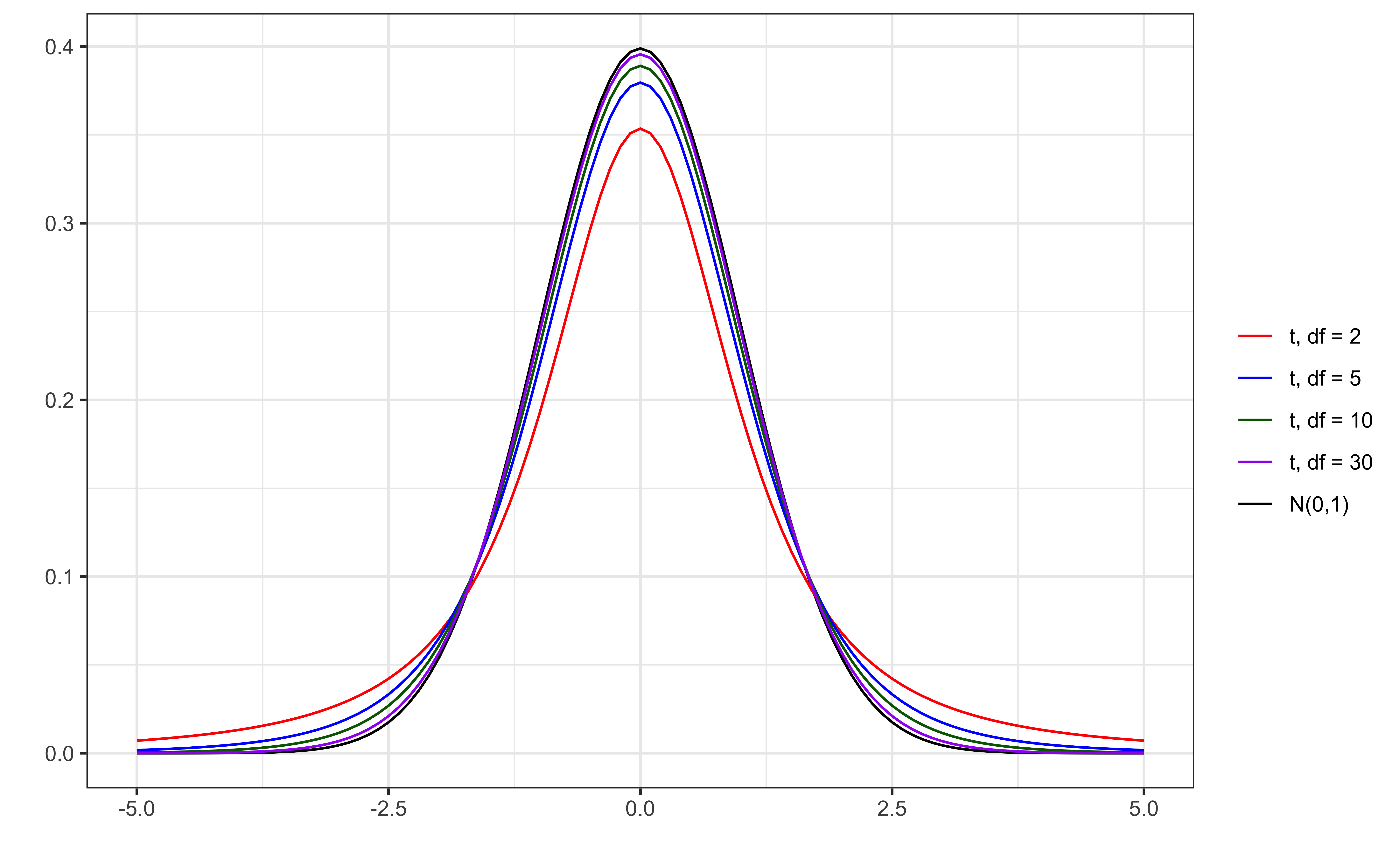
Figure 1: Standard normal vs. t distributions

Hypothesis test for \(\beta_j\): P-value

The p-value measures how likely it is to see results at least as extreme as the observed result, given the null hypothesis is true.

\[ \text{p-value} = P(|t| > |T|), \]

calculated from a \(t\) distribution with \(n- p - 1\) degrees of freedom

Why do we take into account the high and low ends of the distribution to define “extreme” for this test?

Understanding the p-value

Magnitude of p-value	Interpretation
p-value < 0.01	strong evidence against \(H_0\)
0.01 < p-value < 0.05	moderate evidence against \(H_0\)
0.05 < p-value < 0.1	weak evidence against \(H_0\)
p-value > 0.1	effectively no evidence against \(H_0\)

These are general guidelines. The strength of evidence depends on the context of the problem.

Hypothesis test for \(\beta_j\): Conclusion

There are two parts to the conclusion

• Make a conclusion by comparing the p-value to a predetermined decision-making threshold called the significance level ( \(\alpha\) level)

  • If \(\text{p-value} < \alpha\): Reject \(H_0\)

  • If \(\text{p-value} \geq \alpha\): Fail to reject \(H_0\)

• State the conclusion in the context of the data

Application exercise

📋 sta221-sp26.github.io/ae/ae-03-inference

Part 2

Confidence interval for \(\beta_j\)

Confidence interval for \(\beta_j\)

• A plausible range of values for a population parameter is called a confidence interval

• Using only a single point estimate is like fishing in a murky lake with a spear, and using a confidence interval is like fishing with a net

  • We can throw a spear where we saw a fish but we will probably miss, if we toss a net in that area, we have a good chance of catching the fish

  • Similarly, if we report a point estimate, we probably will not hit the exact population parameter, but if we report a range of plausible values we have a good shot at capturing the parameter

What “confidence” means

• We will construct \(C\%\) confidence intervals.

  • The confidence level impacts the width of the interval

• “Confident” means if we were to take repeated samples of the same size as our data, fit regression lines using the same predictors, and calculate \(C\%\) CIs for the coefficient of \(x_j\), then \(C\%\) of those intervals will contain the true value of the coefficient \(\beta_j\)

• Balance precision and accuracy when selecting a confidence level

What is the probability \(\beta_j\) is in the 95% confidence interval

• pre data collection?

• post data collection?

Confidence interval for \(\beta_j\)

\[ \text{Estimate} \pm \text{ (critical value) } \times \text{SE} \]

\[ \hat{\beta}_1 \pm t^* \times SE({\hat{\beta}_j}) \]

where \(t^*\) is calculated from a \(t\) distribution with \(n-p-1\) degrees of freedom

Confidence interval: Critical value

# confidence level: 95%
qt(0.975, df = nrow(football) - 2 - 1)

[1] 1.97928

# confidence level: 90%
qt(0.95, df = nrow(football) - 2 - 1)

[1] 1.657235

# confidence level: 99%
qt(0.995, df = nrow(football) - 2 - 1)

[1] 2.61606

95% CI for \(\beta_j\): Calculation

term	estimate	std.error	statistic	p.value
(Intercept)	19.332	2.984	6.478	0
enrollment_th	0.780	0.110	7.074	0
typePublic	-13.226	3.153	-4.195	0

95% CI for \(\beta_j\) in R

tidy(exp_fit, conf.int = TRUE, conf.level = 0.95) |> 
  kable(digits = 3)

term	estimate	std.error	statistic	p.value	conf.low	conf.high
(Intercept)	19.332	2.984	6.478	0	13.426	25.239
enrollment_th	0.780	0.110	7.074	0	0.562	0.999
typePublic	-13.226	3.153	-4.195	0	-19.466	-6.986

Interpretation: We are 95% confident that for each additional 1,000 students enrolled, the institution’s expenditures on football will be greater by $562,000 to $999,000, on average, holding institution type constant.

Confidence intervals & hypothesis tests

• A \(C\%\) confidence interval corresponds to a two-sided hypothesis test with \(\alpha\)-level of \((100 - C)\%\)

• Using a confidence interval for a two-sided test:

  • If the hypothesized value is in the interval \(\Rightarrow\) Fail to reject \(H_0\)

  • If the hypothesized value is not in the interval \(\Rightarrow\) Reject \(H_0\)

The 95% confidence interval for typePublic is -19.466 to -6.986. Do we reject or fail to reject the null hypothesis that \(\beta_{\text{typePublic}} = 0\) ?

Recap

• Conducted a hypothesis test for a coefficient \(\beta_j\)

• Constructed and interpreted a confidence interval for a coefficient \(\beta_j\)

Next class

• Exam 01 review
• No prepare assignment