Multicollinearity

Prof. Maria Tackett

Feb 24, 2026

Announcements

• Project proposal due TODAY at 11:59pm on GitHub

• February 25, 5-6 pm @ East Duke 108: Duke Sports Analytics Club is hosting Sam Marks, Director of Business Strategy and Analytics at the Boston Bruins

  • Click here to register

• SSMU Mini DataFest #2: February 27 - March 1. Click here for announcement

• March 20 - 22: ASA DataFest at Duke

  • Learn more and register: https://dukestatsci.github.io/datafest/#signup 

Computing set up

# load packages
library(tidyverse)  
library(tidymodels)  
library(knitr)       
library(patchwork)
library(GGally)   # for pairwise plot matrix
library(corrplot) # for correlation matrix
# set default theme in ggplot2
ggplot2::theme_set(ggplot2::theme_bw())

Topics

• Model conditions and diagnostics

• Multicollinearity

  • Definition

  • How it impacts the model

  • How to detect it

  • What to do about it

Model conditions and diagnostics

Assumptions for regression

\[ \mathbf{y}|\mathbf{X} \sim N(\mathbf{X}\boldsymbol{\beta}, \sigma_\epsilon^2\mathbf{I}) \]

1. Linearity: There is a linear relationship between the response and predictor variables.
2. Equal variance: The variability about the least squares line is generally constant.
3. Normality: The distribution of the errors (residuals) is approximately normal.
4. Independence: The errors (residuals) are independent from one another.

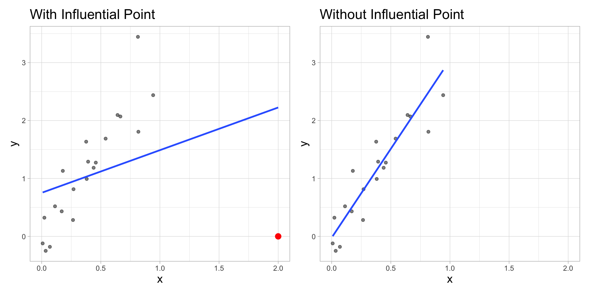
Influential Point

An observation is influential if removing has a noticeable impact on the regression coefficients

Cook’s Distance

Cook’s distance for the \(i^{th}\) observation is

\[ D_i = \frac{r^2_i}{p + 1}\Big(\frac{h_{ii}}{1 - h_{ii}}\Big) \]

where \(r_i\) is the studentized residual and \(h_{ii}\) is the leverage for the \(i^{th}\) observation

This measure is a combination of

• How well the model fits the \(i^{th}\) observation

• How far the \(i^{th}\) observation is from the rest of the data

Using Cook’s Distance

• An observation with large value of \(D_i\) is said to have a strong influence on the predicted values

• General thresholds .An observation with

  • \(D_i > 0.5\) is moderately influential

  • \(D_i > 1\) is very influential

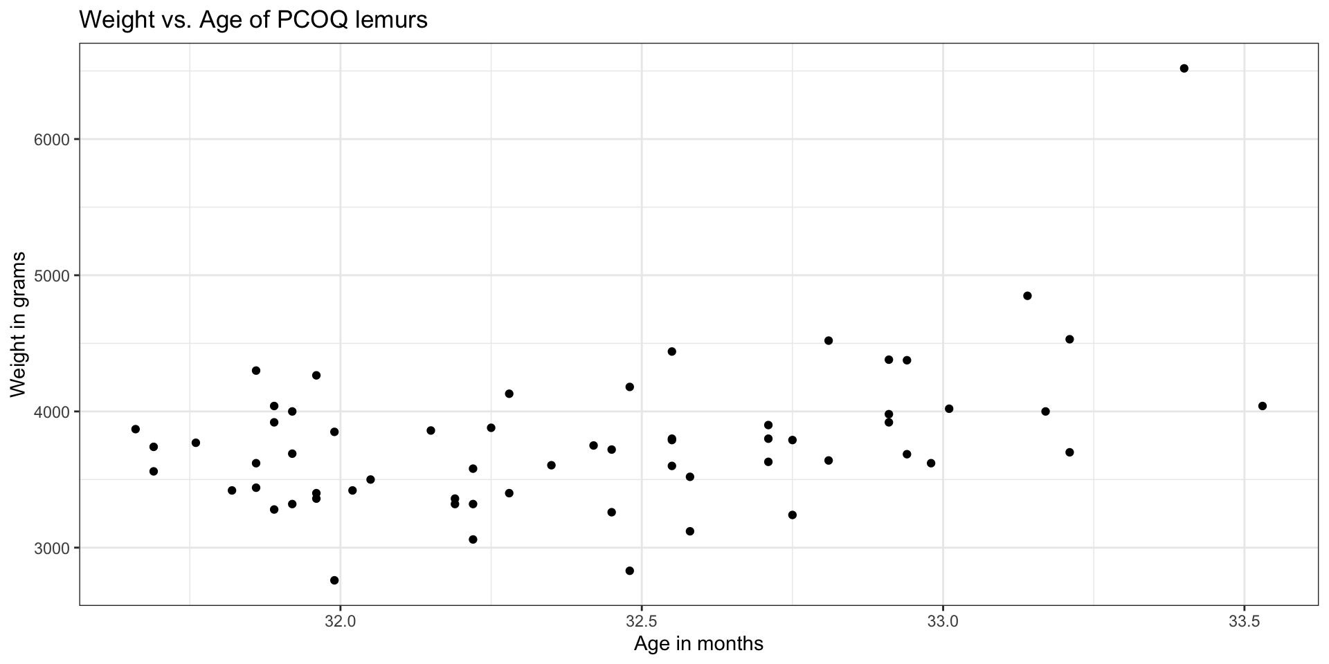
Lemurs data

Large leverage

• Measure of how far the predictor (combination of predictors) is from the typical value (combination)

• The sum of the leverages for all points is \(p + 1\), where \(p\) is the number of predictors in the model . More specifically

  \[ \sum_{i=1}^n h_{ii} = \text{rank}(\mathbf{H}) = \text{rank}(\mathbf{X}) = p+1 \]

• The average value of leverage, \(h_{ii}\), is \(\bar{h} = \frac{(p+1)}{n}\)

• An observation has large leverage if \[h_{ii} > \frac{2(p+1)}{n}\]

Scaled residuals

• What is the best way to identify outlier points that don’t fit the pattern from the regression line?

  • Look for points that have large residuals

• We can rescale residuals and put them on a common scale to more easily identify “large” residuals

• We will consider two types of scaled residuals: standardized residuals and studentized residuals

Standardized residuals

• The variance of the residuals can be estimated by the mean squared residuals (MSR) \(= \frac{SSR}{n - p - 1} = \hat{\sigma}^2_{\epsilon}\)

• We can use MSR to compute standardized residuals

  \[ std.res_i = \frac{e_i}{\sqrt{MSR}} \]

• Standardized residuals are produced by augment() in the column .std.resid

Using standardized residuals

We can examine the standardized residuals directly from the output from the augment() function

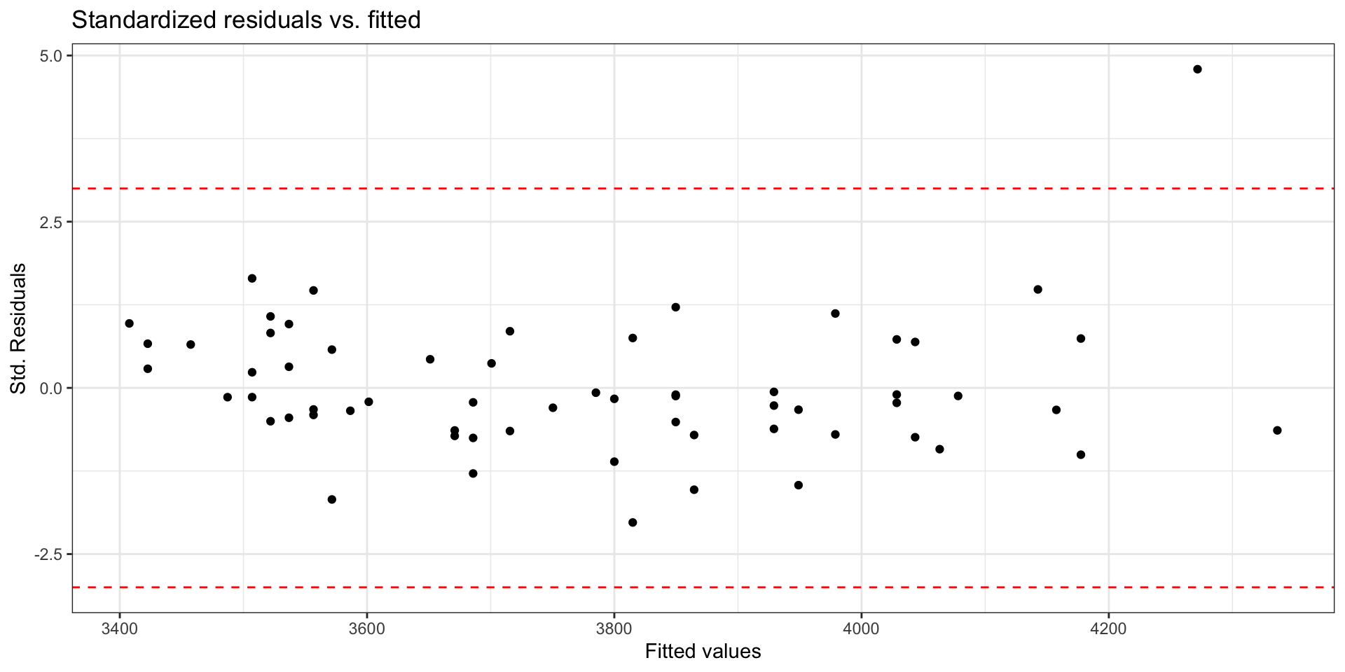
• An observation is a potential outlier if its standardized residual is beyond \(\pm 3\)

Studentized residuals

• MSR is an approximation of the variance of the residuals.

• The variance of the residuals is \(Var(\mathbf{e}) = \sigma^2_{\epsilon}(\mathbf{I} - \mathbf{H})\)

  • The variance of the \(i^{th}\) residual is \(Var(e_i) = \sigma^2_{\epsilon}(1 - h_{ii})\)

• The studentized residual is the residual rescaled by the more exact calculation for variance

\[ r_i = \frac{e_{i}}{\sqrt{\hat{\sigma}^2_{\epsilon}(1 - h_{ii})}} \]

• Standardized and studentized residuals provide similar information about which points are outliers in the response.
  • Studentized residuals are used to compute Cook’s Distance.

Using these measures

• Standardized residuals, leverage, and Cook’s Distance should all be examined together

• Examine plots of the measures to identify observations that are outliers, high leverage, and may potentially impact the model.

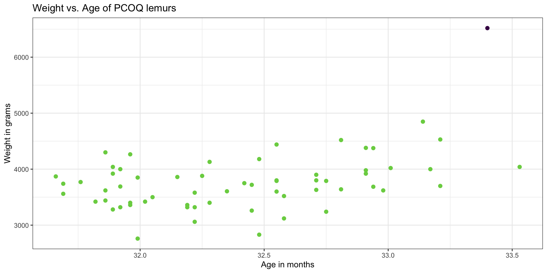
Back to the influential point

What to do with outliers/influential points?

• First consider if the outlier is a result of a data entry error.

• If not, you may consider dropping an observation if it’s an outlier in the predictor variables if…

  • It is meaningful to drop the observation given the context of the problem

  • You intended to build a model on a smaller range of the predictor variables. Mention this in the write up of the results and be careful to avoid extrapolation when making predictions

What to do with outliers/influential points?

• It is generally not good practice to drop observations that ar outliers in the value of the response variable

  • These are legitimate observations and should be in the model

  • You can try transformations or increasing the sample size by collecting more data

• A general strategy when there are influential points is to fit the model with and without the influential points and compare the outcomes

Multicollinearity

Data: Trail users

• The Pioneer Valley Planning Commission (PVPC) collected data at the beginning a trail in Florence, MA for ninety days from April 5, 2005 to November 15, 2005 to
• Data collectors set up a laser sensor, with breaks in the laser beam recording when a rail-trail user passed the data collection station.

# A tibble: 5 × 7
  volume hightemp avgtemp season cloudcover precip day_type
   <dbl>    <dbl>   <dbl> <chr>       <dbl>  <dbl> <chr>   
1    501       83    66.5 Summer       7.60  0     Weekday 
2    419       73    61   Summer       6.30  0.290 Weekday 
3    397       74    63   Spring       7.5   0.320 Weekday 
4    385       95    78   Summer       2.60  0     Weekend 
5    200       44    48   Spring      10     0.140 Weekday 

Source: Pioneer Valley Planning Commission via the mosaicData package.

Variables

Response

• volume estimated number of trail users that day (number of breaks recorded)

Predictors

• hightemp daily high temperature (in degrees Fahrenheit)

• avgtemp average of daily low and daily high temperature (in degrees Fahrenheit)

• season one of “Fall”, “Spring”, or “Summer”

• precip measure of precipitation (in inches)

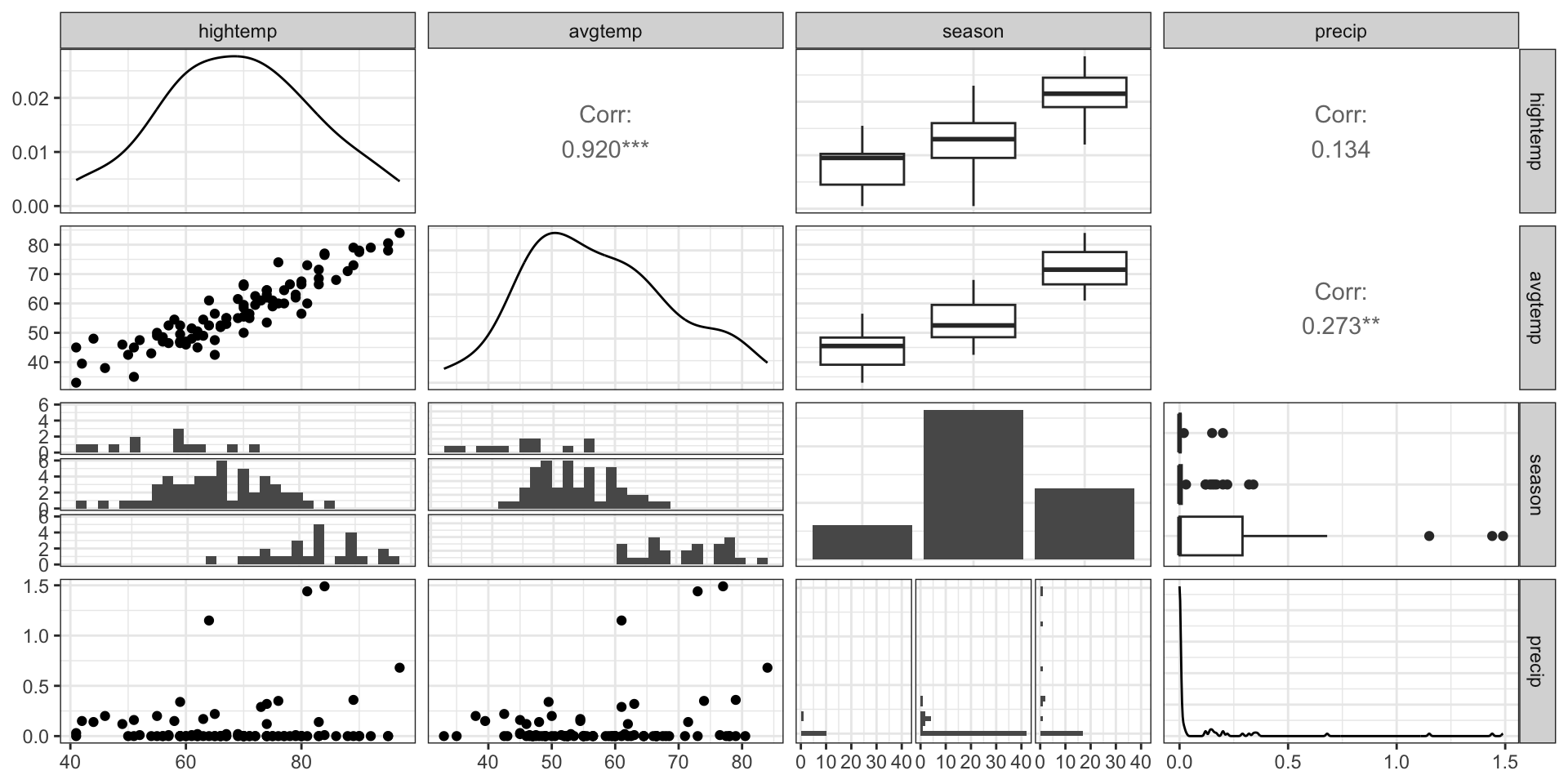
EDA: Relationship between predictors

We can create a pairwise plot matrix using the ggpairs function from the GGally R package

rail_trail |>
  select(hightemp, avgtemp, season, precip) |>
  ggpairs()

EDA: Relationship between predictors

EDA: Correlation matrix

We can. use corrplot() in the corrplot R package to make a matrix of pairwise correlations between quantitative predictors

correlations <- rail_trail |>
  select(hightemp, avgtemp, precip) |>
  cor()

corrplot(correlations, method = "number")

EDA: Correlation matrix

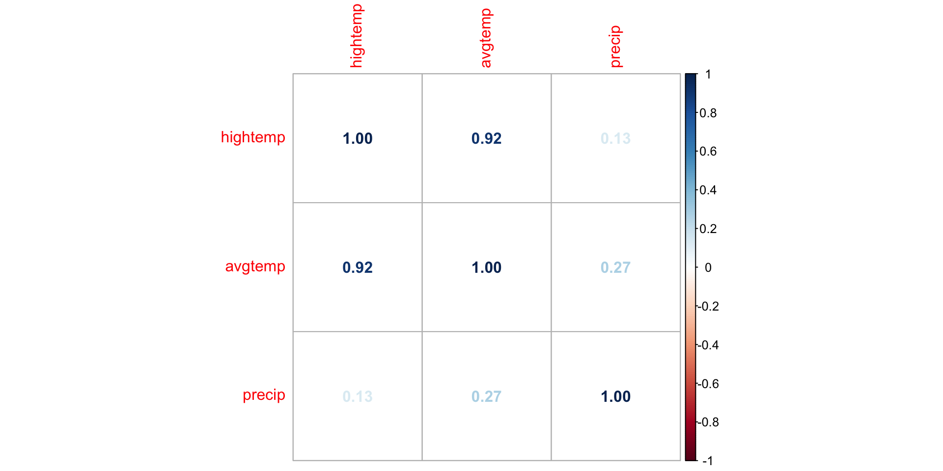
What might be a potential concern with a model that uses high temperature, average temperature, season, and precipitation to predict volume?

Multicollinearity

Multicollinearity

• Ideally the predictors are orthogonal, meaning they are completely independent of one another

• In practice, there is typically some dependence between predictors but it is often not a major issue in the model

• If there is linear dependence among (a subset of) the predictors, we cannot find \(\hat{\boldsymbol{\beta}}\)

• If there are near-linear dependencies, we can find \(\hat{\boldsymbol{\beta}}\) but there may be other issues with the model

• Multicollinearity: near-linear dependence among predictors

Sources of multicollinearity

• Data collection method - only sample from a subspace of the region of predictors

• Constraints in the population - e.g., predictors family income and size of house

• Choice of model - e.g., adding high order terms to the model

• Overdefined model - have more predictors than observations

Source: Montgomery, Peck, and Vining (2021)

Detecting multicollinearity

• Recall \(Var(\hat{\boldsymbol{\beta}}) = \sigma^2_{\epsilon}(\mathbf{X}^\mathsf{T}\mathbf{X})^{-1}\)
• Let \(\mathbf{C} = (\mathbf{X}^\mathsf{T}\mathbf{X})^{-1}\). Then \(Var(\hat{\beta}_j) = \sigma^2_{\epsilon}C_{jj}\)
• When there are near-linear dependencies, \(C_{jj}\) increases and thus \(Var(\hat{\beta}_j)\) becomes inflated
• \(C_{jj}\) is associated with how much \(Var(\hat{\beta}_j)\) is inflated due to \(x_j\) dependencies with other predictors

Variance inflation factor

• The variance inflation factor (VIF) measures how much the linear dependencies impact the variance of the predictors

\[ VIF_{j} = \frac{1}{1 - R^2_j} \]

where \(R^2_j\) is the proportion of variation in \(x_j\) that is explained by a linear combination of all the other predictors

• When the response and predictors are scaled in a particular way, \(C_{jj} = VIF_{j}\). Click here to see how.

Detecting multicollinearity

• Common practice uses threshold \(VIF > 10\) as indication of concerning multicollinearity (some say VIF > 5 is worth investigation)

• Variables with similar values of VIF are typically the ones correlated with each other

• Use the vif() function in the rms R package to calculate VIF

library(rms)

trail_fit <- lm(volume ~ hightemp + avgtemp + precip, data = rail_trail)

vif(trail_fit)

hightemp  avgtemp   precip 
7.161882 7.597154 1.193431 

How multicollinearity impacts model

• Large variance for the model coefficients that are collinear

  • Different combinations of coefficient estimates produce equally good model fits

• Unreliable statistical inference results

  • May conclude coefficients are not statistically significant when there is, in fact, a relationship between the predictors and response

• Interpretation of coefficient is no longer “holding all other variables constant”, since this would be impossible for correlated predictors

Application exercise

📋 sta221-sp26.github.io/ae/ae-04-multicollinearity.html

Part 1

Dealing with multicollinearity

• Collect more data (often not feasible given practical constraints)

• Redefine the correlated predictors to keep the information from predictors but eliminate collinearity

  • e.g., if \(x_1, x_2, x_3\) are correlated, use a new variable \((x_1 + x_2) / x_3\) in the model

• For categorical predictors, avoid using levels with very few observations as the baseline

• Remove one of the correlated variables

  • Be careful about substantially reducing predictive power of the model

Application exercise

📋 sta221-sp26.github.io/ae/ae-04-multicollinearity.html

Part 2

Recap

• Reviewed model conditions and diagnostics

• Introduced multicollinearity and how it impacts a model

Next class

• Variable transformations

• Complete Lecture 13 prepare

References

Montgomery, Douglas C, Elizabeth A Peck, and G Geoffrey Vining. 2021. Introduction to Linear Regression Analysis. John Wiley & Sons.