Variable transformations
Feb 26, 2026
Announcements
SSMU Mini DataFest #2: February 27 - March 1. Click here for announcement
March 20 - 22: ASA DataFest at Duke
- Learn more and register: https://dukestatsci.github.io/datafest/#signup
Computing set up
Topics
- Log-transformation on the response variable
- Log-transformation on predictor variable(s)
- Identifying linear models
Variable transformations
Data: Life expectancy in 140 countries
The data set comes from Zarulli et al. (2021) who analyze the effects of a country’s healthcare expenditures and other factors on the country’s life expectancy. The data are originally from the Human Development Database and World Health Organization.
There are 140 countries (observations) in the data set.
Variables
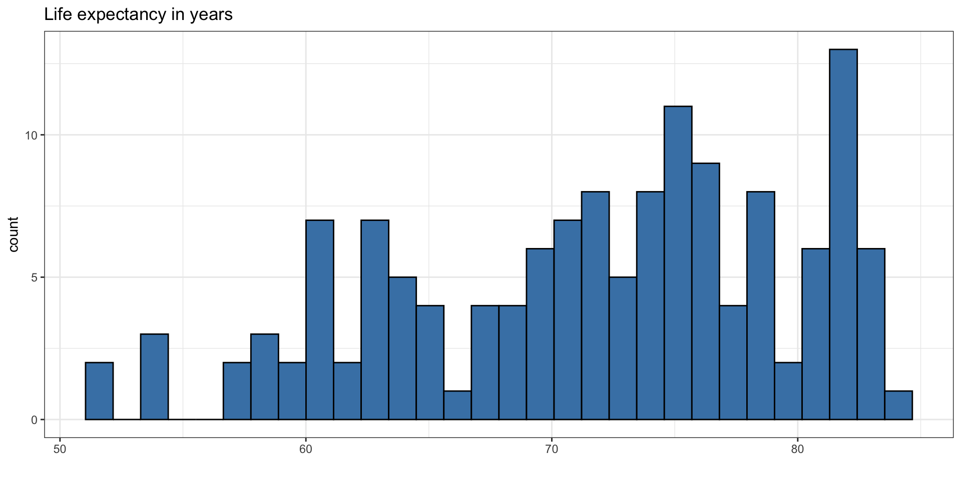
life_exp: The average number of years that a newborn could expect to live, if he or she were to pass through life exposed to the sex- and age-specific death rates prevailing at the time of his or her birth, for a specific year, in a given country, territory, or geographic income_inequality. ( from the World Health Organization)income_inequality: Measure of the deviation of the distribution of income among individuals or households within a country from a perfectly equal distribution. A value of 0 represents absolute equality, a value of 100 absolute inequality (based on Gini coefficient). (from Zarulli et al. (2021))
Variables
education: Indicator of whether a country’s education index is above (High) or below (Low) the median index for the 140 countries in the data set.- Education index: Average of mean years of schooling (of adults) and expected years of school (of children), both expressed as an index obtained by scaling wit the corresponding maxima.
health_expend: Per capita current spending on on healthcare goods and services, expressed in respective currency - international Purchasing Power Parity (PPP) dollar (from the World Health Organization)
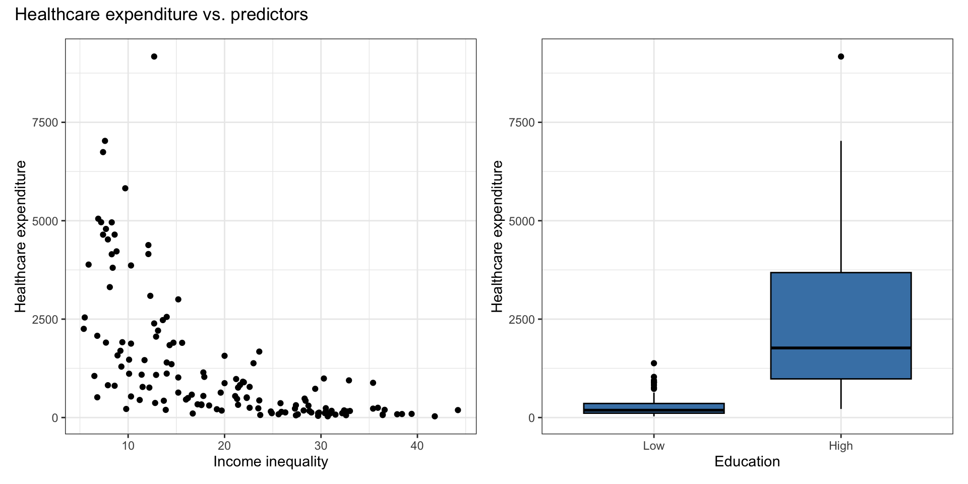
Exploratory data analysis
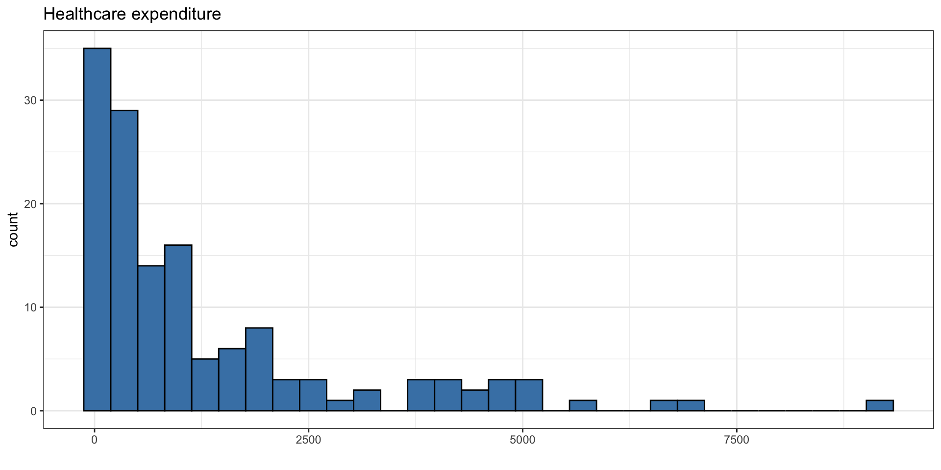
Exploratory data analysis
The goal is to use income inequality and education to understand variability in healthcare expenditure.
Original model
| term | estimate | std.error | statistic | p.value |
|---|---|---|---|---|
| (Intercept) | 2070.599 | 534.653 | 3.873 | 0.000 |
| income_inequality | -64.346 | 18.626 | -3.455 | 0.001 |
| educationHigh | 1039.298 | 359.736 | 2.889 | 0.004 |
Original model: Residuals vs. fitted

What model assumption(s) appear to be violated?
Consider different transformations…
Transformation on \(\mathbf{y}\)
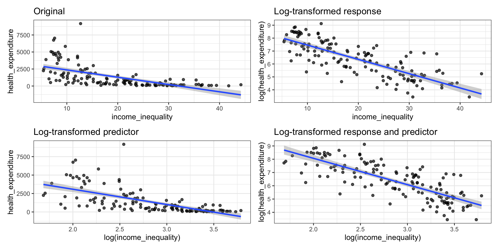
Identifying a need to transform \(\mathbf{y}\)
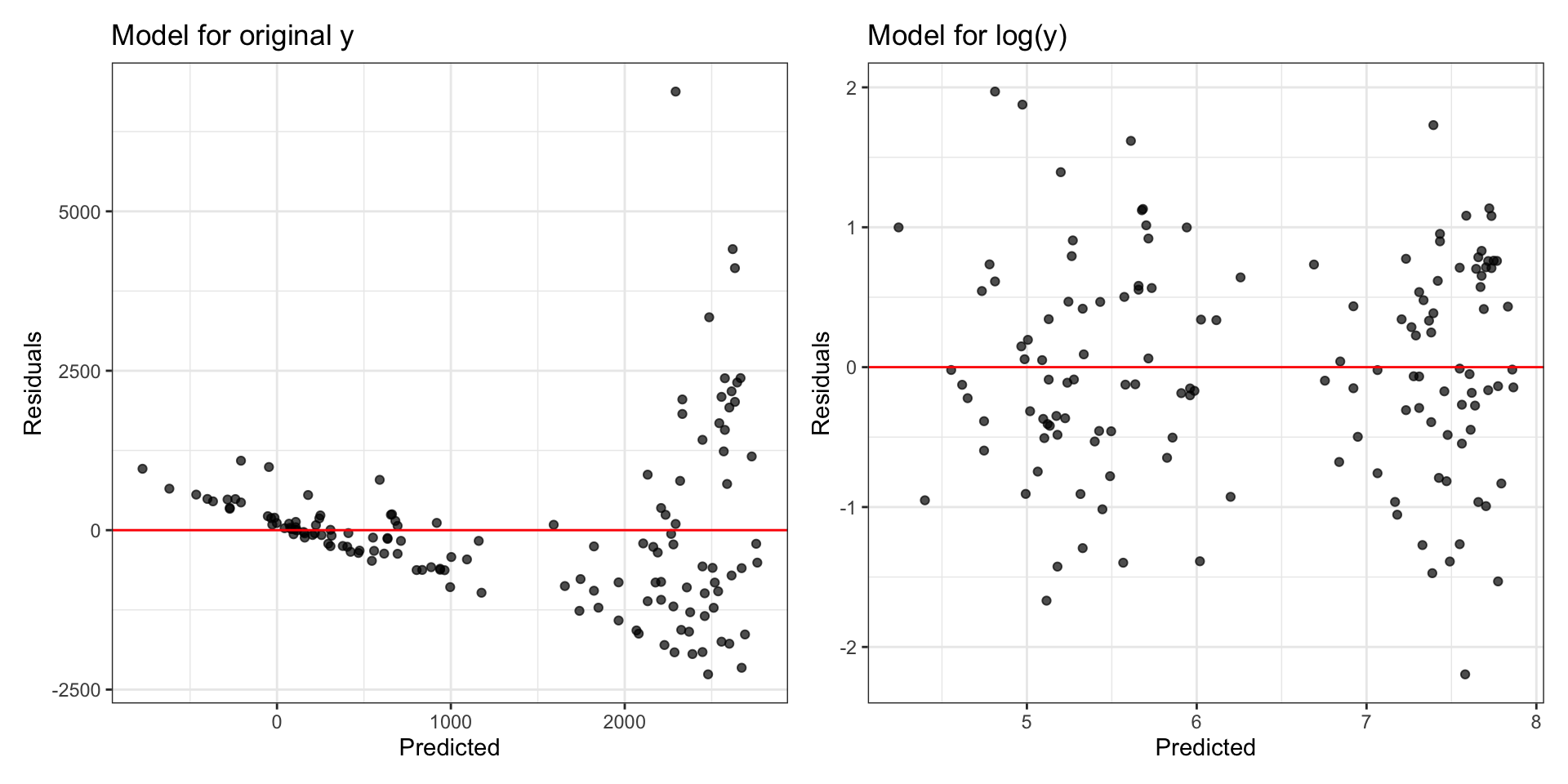
Typically, a “fan-shaped” residual plot indicates the need for a transformation on \(\mathbf{y} = [y_1 \dots y_n]^\mathsf{T}\)
There are multiple ways to transform the values of the response, e.g., \(\sqrt{y_i}\), \(1/ y_i\), \(\log(y_i)\). These are called variance stabilizing transformations.
\(\log(y_i)\) the most straightforward to interpret, so we use that transformation when possible
When building a model:
Choose a transformation and build the model on the transformed data
Reassess the residual plots
If the residuals plots did not sufficiently improve, try a new transformation!
Log transformation on \(\mathbf{y}\)
- If we apply a log transformation to the response variable, we want to estimate the parameters for the statistical model
\[ \log(\mathbf{y}) = \mathbf{X}\boldsymbol{\beta} + \boldsymbol{\epsilon}, \quad \boldsymbol{\epsilon} \sim N(\mathbf{0}, \sigma^2_{\epsilon}\mathbf{I}) \]
- The regression equation is
\[\widehat{\log(\mathbf{y})} = \mathbf{X}\hat{\boldsymbol{\beta}}\]
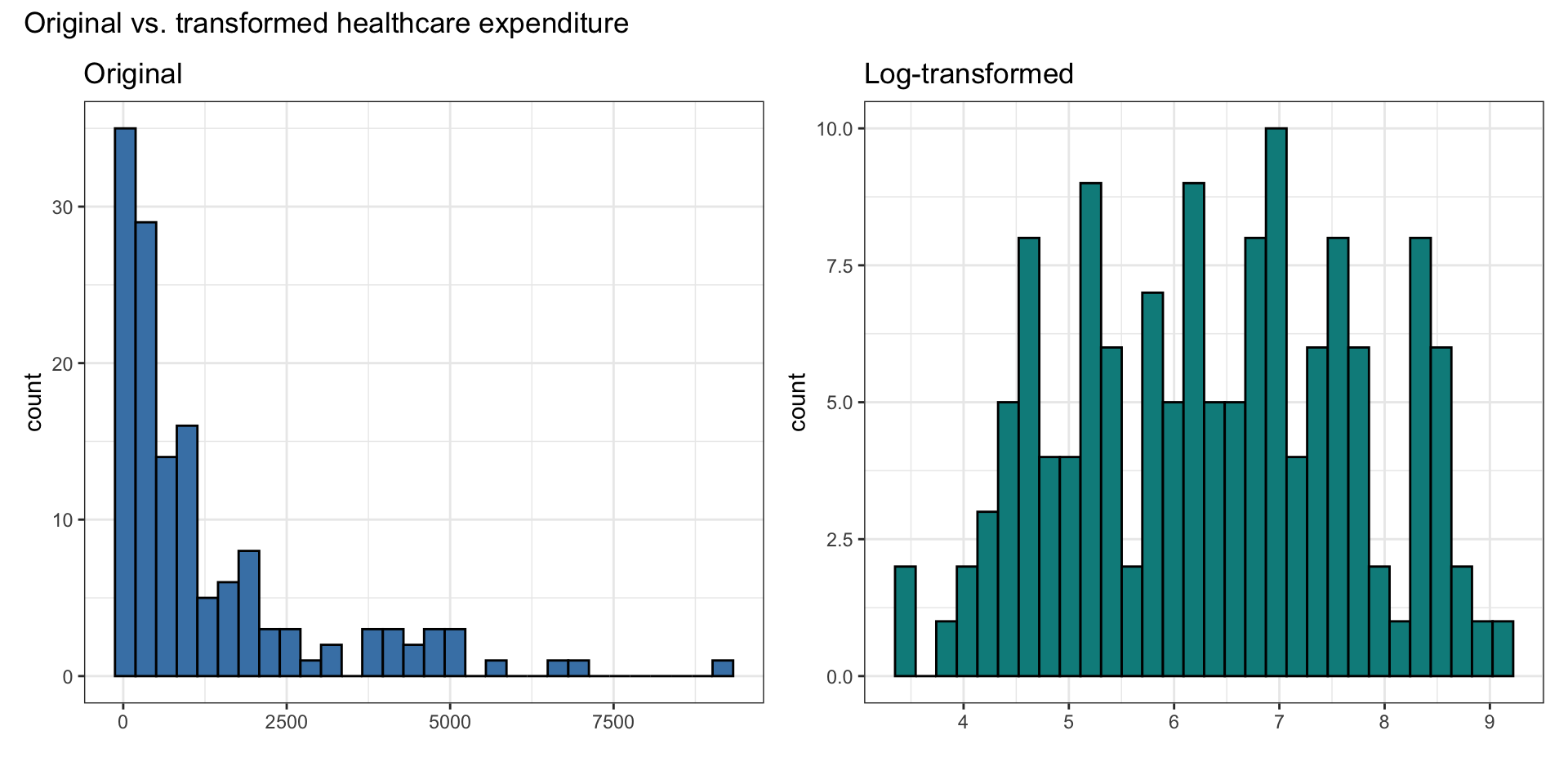
Distribution of \(\mathbf{y}\) and \(\log(\mathbf{y})\)
Model with \(\log(\mathbf{y})\)
| term | estimate | std.error | statistic | p.value |
|---|---|---|---|---|
| (Intercept) | 7.096 | 0.324 | 21.895 | 0 |
| income_inequality | -0.065 | 0.011 | -5.714 | 0 |
| educationHigh | 1.117 | 0.218 | 5.121 | 0 |
Model with \(\log(\mathbf{y})\): Residuals
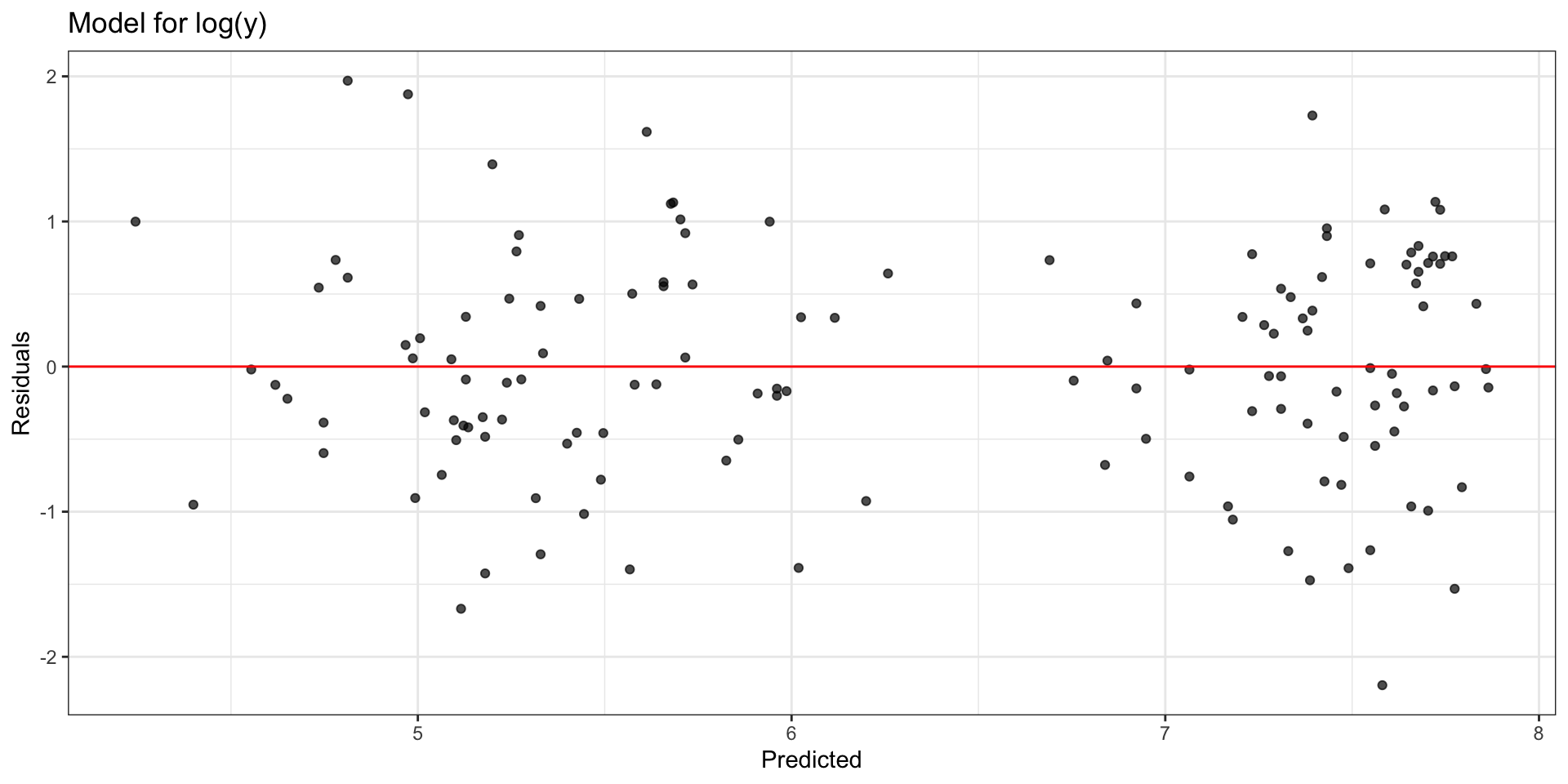
Compare residual plots
Model interpretation in terms of \(\mathbf{y}\)
Let \(\mathbf{x}_i^\mathsf{T}\) be the \(i^{th}\) row of \(\mathbf{X}\). Then,
\[\begin{align} \widehat{\log(y_i)} &= \mathbf{x}_i^\mathsf{T}\hat{\boldsymbol{\beta}}\\ \Rightarrow \hat{y_i} &= e^{\mathbf{x}^\mathsf{T}_i\hat{\boldsymbol{\beta}}} \\ & = e^{(\hat{\beta}_0 + \hat{\beta}_1 x_{i1} + \dots + \hat{\beta}_px_{ip})} \\ &= e^{\hat{\beta}_0}e^{\hat{\beta}_1x_{i1}}\dots e^{\hat{\beta}_px_{ip}}\end{align}\]
Intercept: When \(x_{i1} = \dots = x_{ip} =0\), \(y_i\) is expected to be \(e^{\hat{\beta}_0}\)
Coefficient of \(X_j\): For every one unit increase in \(x_{ij}\), \(y_{i}\) is expected to multiply by a factor of \(e^{\hat{\beta}_j}\), holding all else constant.
Interpretation
| term | estimate | std.error | statistic | p.value |
|---|---|---|---|---|
| (Intercept) | 7.096 | 0.324 | 21.895 | 0 |
| income_inequality | -0.065 | 0.011 | -5.714 | 0 |
| educationHigh | 1.117 | 0.218 | 5.121 | 0 |
Interpret each of the following in terms of healthcare expenditure
Intercept
income_inequalityeducation
Transformation on \(x_j\)
Variability in life expectancy
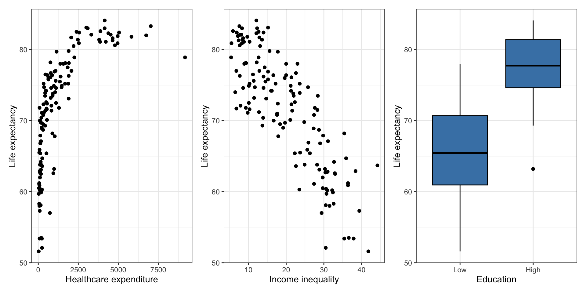
Let’s consider a model using a country’s healthcare expenditure, income inequality, and education understand variability in its life expectancy.
Bivariate EDA
Original model
| term | estimate | std.error | statistic | p.value |
|---|---|---|---|---|
| (Intercept) | 78.575 | 1.775 | 44.274 | 0.000 |
| health_expenditure | 0.001 | 0.000 | 4.522 | 0.000 |
| income_inequality | -0.484 | 0.061 | -7.900 | 0.000 |
| educationHigh | 2.020 | 1.168 | 1.730 | 0.086 |
Original model: Residuals
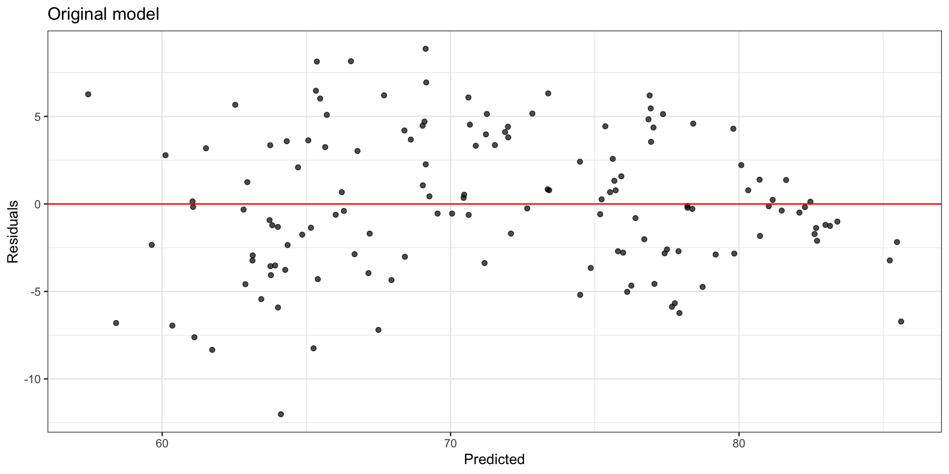
Look at residuals vs. each predictor to determine which variable has non-linear relationship with life expectancy.
Residuals vs. predictors
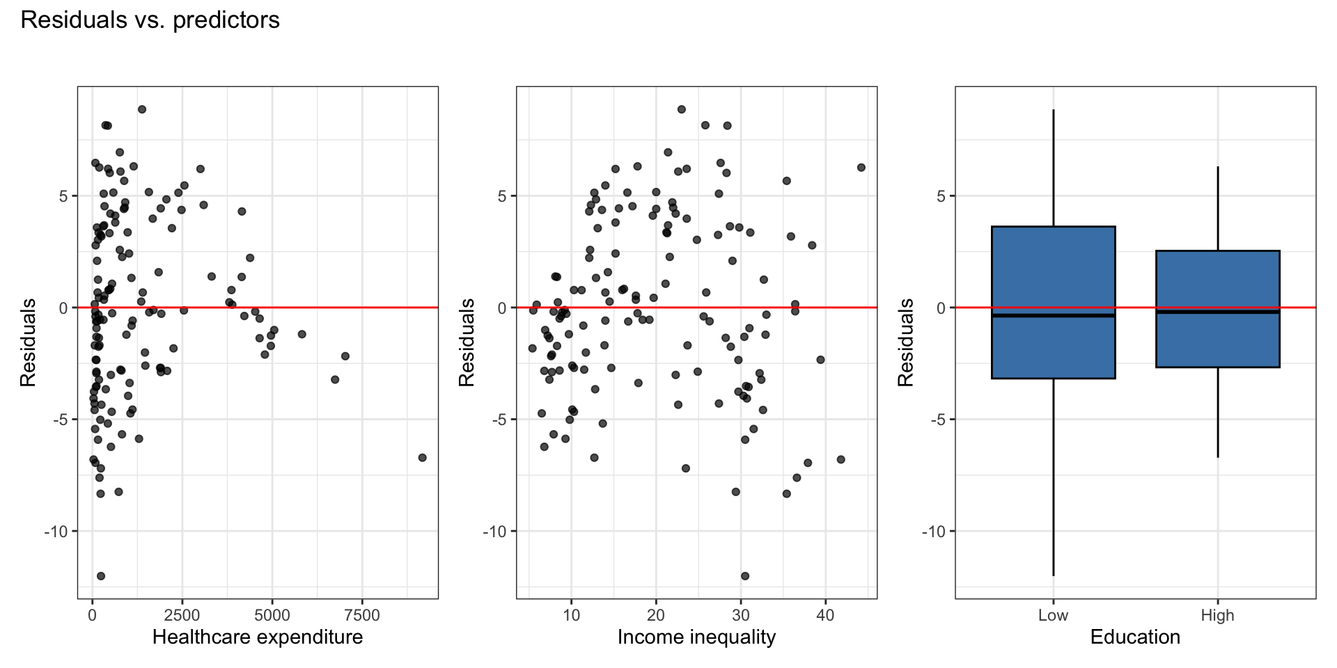
There is a non-linear relationship is between healthcare expenditure and life expectancy.
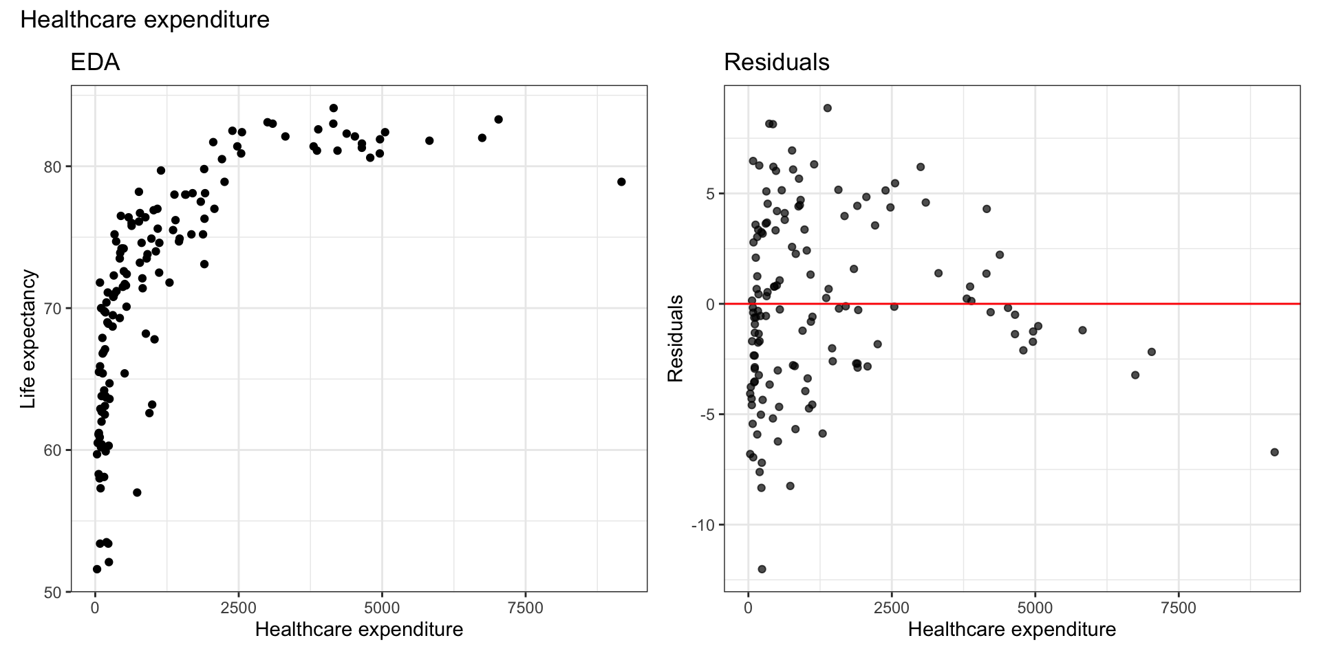
Log Transformation on \(x_j\)
Consider a transformation on predictor \(x_j\) if the scatterplot in EDA shows non-linear relationship and residuals vs. fitted looks parabolic
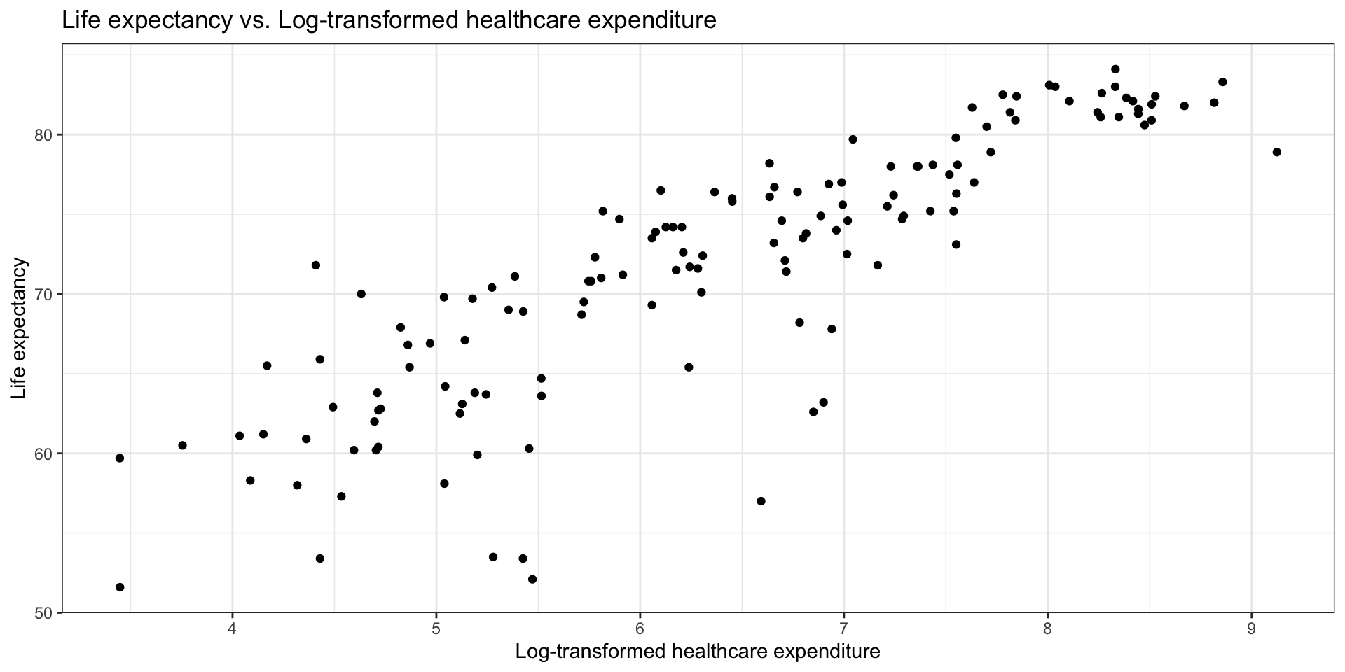
Bivariate EDA with log(health_expend)
Model with Transformation on \(x_j\)
When we fit a model with predictor \(\log(x_j)\), we fit a model of the form
\[ \mathbf{y} = \mathbf{X}\boldsymbol{\beta} + \boldsymbol{\epsilon}, \quad \boldsymbol{\epsilon} \sim N(\mathbf{0}, \sigma^2_{\epsilon}\mathbf{I}) \]
such that \(\mathbf{X}\) has a column for \(\log(x_j)\) .
The estimated regression model is
\[ \begin{aligned} \hat{\mathbf{y}} &= \mathbf{X}\hat{\boldsymbol{\beta}} \\[8pt] \Rightarrow \quad &\hat{y}_i = \hat{\beta}_0 + \hat{\beta}_1x_{i1} + \ldots + \hat{\beta}_j\log(x_{ij}) + \dots + \hat{\beta}_px_{ip} \end{aligned} \]
Model with \(\log(x_j)\)
| term | estimate | std.error | statistic | p.value |
|---|---|---|---|---|
| (Intercept) | 59.151 | 3.184 | 18.576 | 0.000 |
| log(health_expenditure) | 3.092 | 0.396 | 7.814 | 0.000 |
| income_inequality | -0.362 | 0.058 | -6.225 | 0.000 |
| educationHigh | -0.168 | 1.103 | -0.152 | 0.879 |
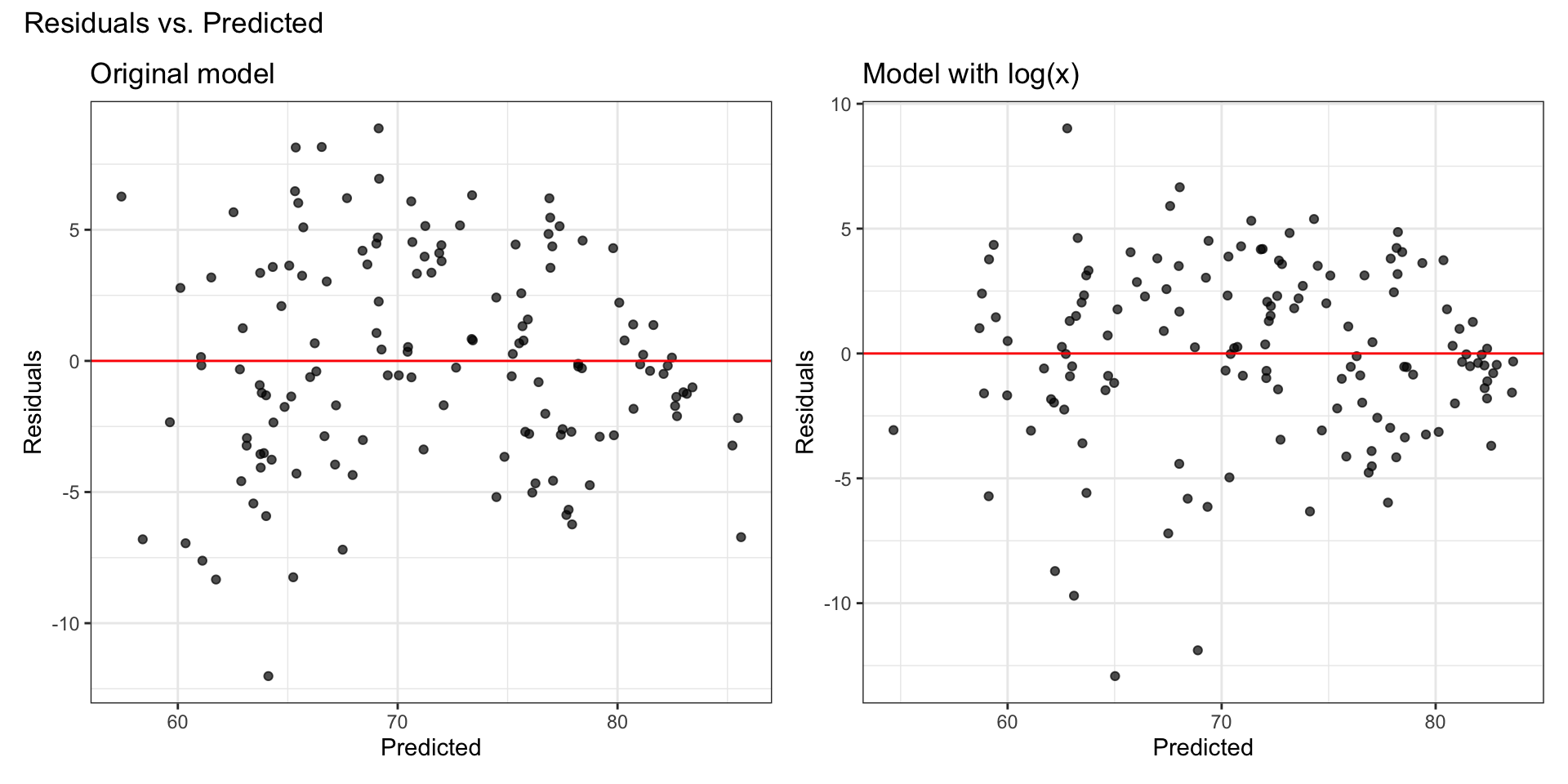
Model with \(\log(x_j)\): Residuals
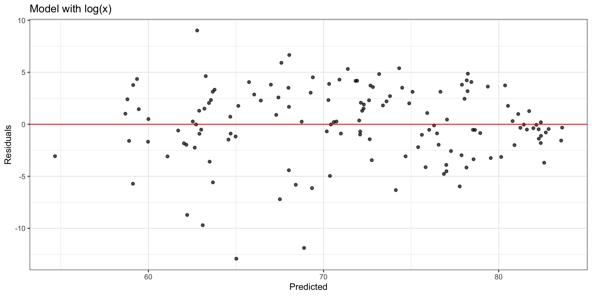
Comparing residual plots
Model interpretation
\[ \hat{y}_i = \hat{\beta}_0 + \hat{\beta}_1x_{i1} + \ldots + \hat{\beta}_j\log(x_{ij}) + \dots + \hat{\beta}_px_{ip} \]
Intercept: When \(x_{i1} = \dots = \log(x_{ij}) = \dots = x_{ip} = 0\) , \(y_i\) is expected to be \(\hat{\beta}_0\), on average.
- \(\log(x_{ij}) = 0\) when \(x_{ij} = 1\)
Coefficient of \(x_j\): When \(x_{ij}\) is multiplied by a factor of \(C\), \(y_i\) is expected to change by \(\hat{\beta}_j\log(C)\) units, on average, holding all else constant.
- Example: When \(x_{ij}\) is multiplied by a factor of 2, \(y_i\) is expected to increase by \(\hat{\beta}_j\log(2)\) units, on average, holding all else constant.
Model with \(\log(x_j)\)
| term | estimate | std.error | statistic | p.value |
|---|---|---|---|---|
| (Intercept) | 59.151 | 3.184 | 18.576 | 0.000 |
| log(health_expenditure) | 3.092 | 0.396 | 7.814 | 0.000 |
| income_inequality | -0.362 | 0.058 | -6.225 | 0.000 |
| educationHigh | -0.168 | 1.103 | -0.152 | 0.879 |
Interpret the intercept in the context of the data.
Interpret the effect of a 10% increase in healthcare expenditure in the context of the data.
Interpret the effect of education in the context of the data.
Linear model
Is a model with log-transformed response and/or predictor still a “linear” model?
“Linear” model
What does it mean for a model to be a “linear” model?
Linear models are linear in the parameters, i.e. given an observation \(y_i\)
\[ y_i = \beta_0 + \beta_1f_1(x_{i1}) + \dots + \beta_pf_p(x_{ip}) + \epsilon_i \]
The functions \(f_1, \ldots, f_p\) can be non-linear as long as \(\beta_0, \beta_1, \ldots, \beta_p\) are linear (additive and not transformed)
Identify the linear models
\(y_i = \beta_0 + \beta_1x_{i1} + \beta_2x_{i1}^2 + \beta_3x_{i2} + \epsilon_i\)
\(y_i = \beta_1x_{i1} + \beta_2x_{i2} + \beta_3x_{i1}x_{i2} + \epsilon_i\)
\(y_i = \beta_0 + \beta_1\sin(x_{i1} + \beta_2x_{i2}) + \beta_3x_{i3} + \epsilon_i\)
\(y_i = \beta_0 + \beta_1e^{x_{i1}} + \beta_2e^{x_{i2}} + \epsilon_i\)
\(y_i =e^{(\beta_0 + \beta_1x_{i1} + \beta_2x_{i2} + \beta_3x_{i3})} + \epsilon_i\)
🔗 Submit response: https://forms.office.com/r/sBjWF7jZ05
Recap
- Introduced log-transformation on the response variable
- Introduced log-transformation on predictor variable(s)
- Identified linear models
Next class
Maximum likelihood estimation
Complete Lecture 14 prepare