Logistic Regression

Model selection

Announcements

• Presentation comments due TODAY at 11:59pm

• Statistics experience due April 2 at 11:59pm

• Next project milestone: Draft report due April 10 (before lab)

Presentations

Model selection

Topics

• Comparing models using AIC and BIC

Computational setup

library(tidyverse)
library(tidymodels)
library(pROC)      
library(knitr)
library(kableExtra)

# set default theme in ggplot2
ggplot2::theme_set(ggplot2::theme_bw())

Risk of coronary heart disease

This data set is from an ongoing cardiovascular study on residents of the town of Framingham, Massachusetts. We want to examine the relationship between various health characteristics and the risk of having heart disease.

• high_risk:

  • 1: High risk of having heart disease in next 10 years
  • 0: Not high risk of having heart disease in next 10 years

• age: Age at exam time (in years)

• totChol: Total cholesterol (in mg/dL)

• currentSmoker: 0 = nonsmoker, 1 = smoker

• education: 1 = Some High School, 2 = High School or GED, 3 = Some College or Vocational School, 4 = College

Modeling risk of coronary heart disease

Using age, totChol, and currentSmoker

term	estimate	std.error	statistic	p.value	conf.low	conf.high
(Intercept)	-6.673	0.378	-17.647	0.000	-7.423	-5.940
age	0.082	0.006	14.344	0.000	0.071	0.094
totChol	0.002	0.001	1.940	0.052	0.000	0.004
currentSmoker1	0.443	0.094	4.733	0.000	0.260	0.627

Review: ROC Curve + Model fit

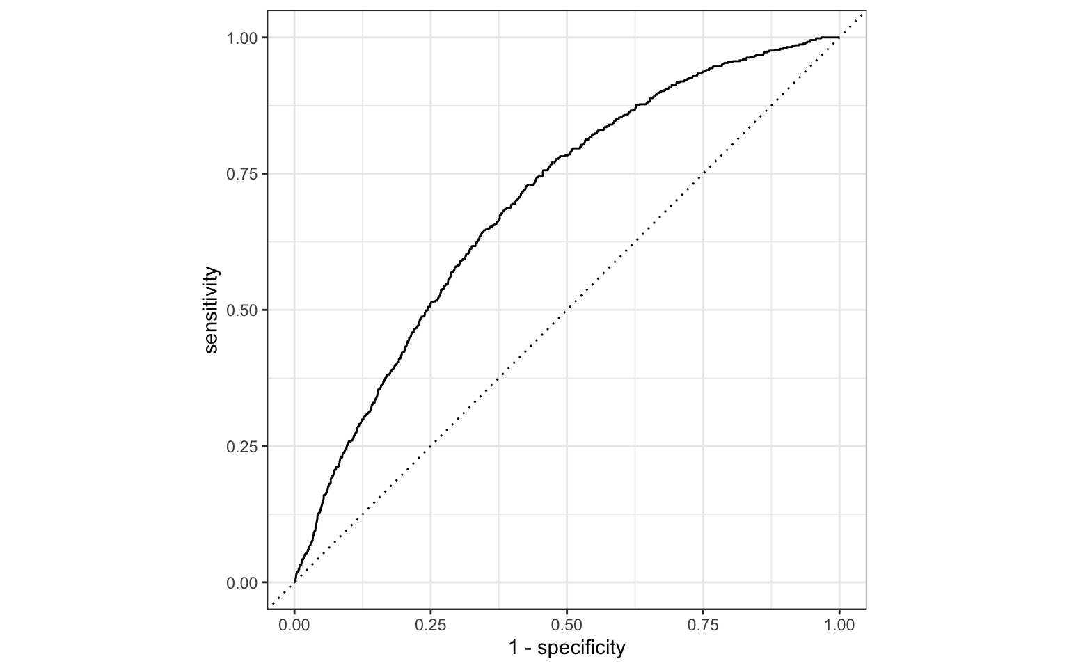
# A tibble: 1 × 3
  .metric .estimator .estimate
  <chr>   <chr>          <dbl>
1 roc_auc binary         0.697

Review: Classification

We will use a threshold of 0.2 to classify observations

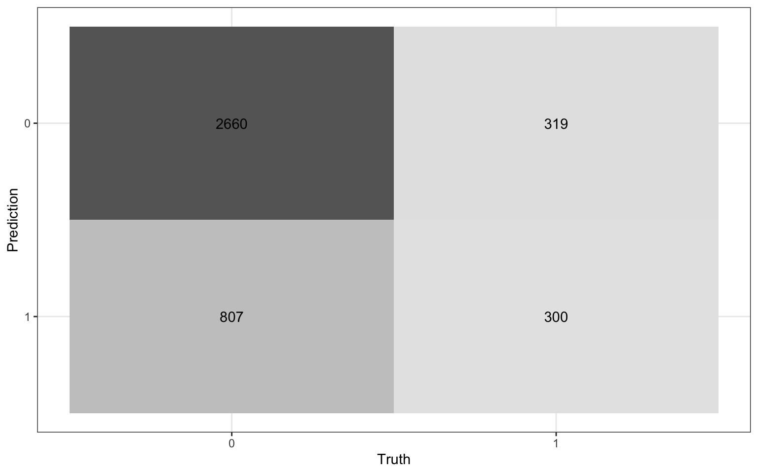
Review: Classification

1. Compute the misclassification rate.

2. Compute sensitivity and explain what it means in the context of the data.

3. Compute specificity and explain what it means in the context of the data.

Model comparison

Which model do we choose?

Model 1

term	estimate
(Intercept)	-6.673
age	0.082
totChol	0.002
currentSmoker1	0.443

Model 2

term	estimate
(Intercept)	-6.456
age	0.080
totChol	0.002
currentSmoker1	0.445
education2	-0.270
education3	-0.232
education4	-0.035

Log-Likelihood

Recall the log-likelihood function

\[ \begin{aligned} \log L&(\boldsymbol{\beta}|x_1, \ldots, x_n, y_1, \dots, y_n) \\ &= \sum\limits_{i=1}^n[y_i \log(\pi_i) + (1 - y_i)\log(1 - \pi_i)] \end{aligned} \]

where \(\pi_i = \frac{\exp\{\mathbf{x}_i^\mathsf{T}\boldsymbol{\beta}\}}{1 + \exp\{\mathbf{x}_i^\mathsf{T}\boldsymbol{\beta}\}}\)

AIC & BIC

Estimators of prediction error and relative quality of models:

. . .

Akaike’s Information Criterion (AIC)¹: \[AIC = -2\log L + 2 (p+1)\]

. . .

Schwarz’s Bayesian Information Criterion (BIC)²: \[ BIC = -2\log L + \log(n)\times(p+1)\]

AIC & BIC

\[ \begin{aligned} & AIC = \color{blue}{-2\log L} \color{black}{+ 2(p+1)} \\ & BIC = \color{blue}{-2\log L} + \color{black}{\log(n)\times(p+1)} \end{aligned} \]

. . .

First Term: Decreases as p increases

AIC & BIC

\[ \begin{aligned} & AIC = -2\log L + \color{blue}{2(p+1)} \\ & BIC = -2\log L + \color{blue}{\log(n)\times (p+1)} \end{aligned} \]

Second term: Increases as p increases

Using AIC & BIC

\[ \begin{aligned} & AIC = -2\log L + \color{red}{2(p+1)} \\ & BIC = -2 \log L + \color{red}{\log(n)\times(p+1)} \end{aligned} \]

• Choose model with the smaller value of AIC or BIC

• If \(n \geq 8\), the penalty for BIC is larger than that of AIC, so BIC tends to favor more parsimonious models (i.e. models with fewer terms)

AIC from the glance() function

Let’s look at the AIC for the model that includes age, totChol, and currentSmoker

glance(high_risk_fit)$AIC

[1] 3232.812

. . .

Calculating AIC

- 2 * glance(high_risk_fit)$logLik + 2 * (3 + 1)

[1] 3232.812

Comparing the models using AIC

Let’s compare the full and reduced models using AIC.

# AIC reduced model 
glance(high_risk_fit_reduced)$AIC

[1] 3232.812

# AIC full model
glance(high_risk_fit_full)$AIC

[1] 3231.6

Based on AIC, which model do you select?

Comparing the models using BIC

Let’s compare the full and reduced models using BIC

# BIC reduced model
glance(high_risk_fit_reduced)$BIC

[1] 3258.074

# BIC full model
glance(high_risk_fit_full)$BIC

[1] 3275.807

Based on BIC, which model do you select?

Recap

• Introduced model selection for logistic regression using

  • AIC and BIC

Next class

• Inference for logistic regression

• Complete Lecture 21 prepare

References

Footnotes

1. Akaike, Hirotugu. “A new look at the statistical model identification.” IEEE transactions on automatic control 19.6 (1974): 716-723.

2. Schwarz, Gideon. “Estimating the dimension of a model.” The annals of statistics (1978): 461-464.