# load packages
library(tidyverse)
library(tidymodels)
library(knitr)
library(kableExtra)
library(patchwork)

# set default theme in ggplot2
ggplot2::theme_set(ggplot2::theme_bw())Inference for regression
Distribution of coefficients
Announcements
HW 02 due Thursday, February 12 at 11:59pm
- Released after class
Exam 01 practice problems + lecture recordings posted on menu of course website
Topics
- Derive distribution of \(\hat{\boldsymbol{\beta}}_j\)
Computing setup
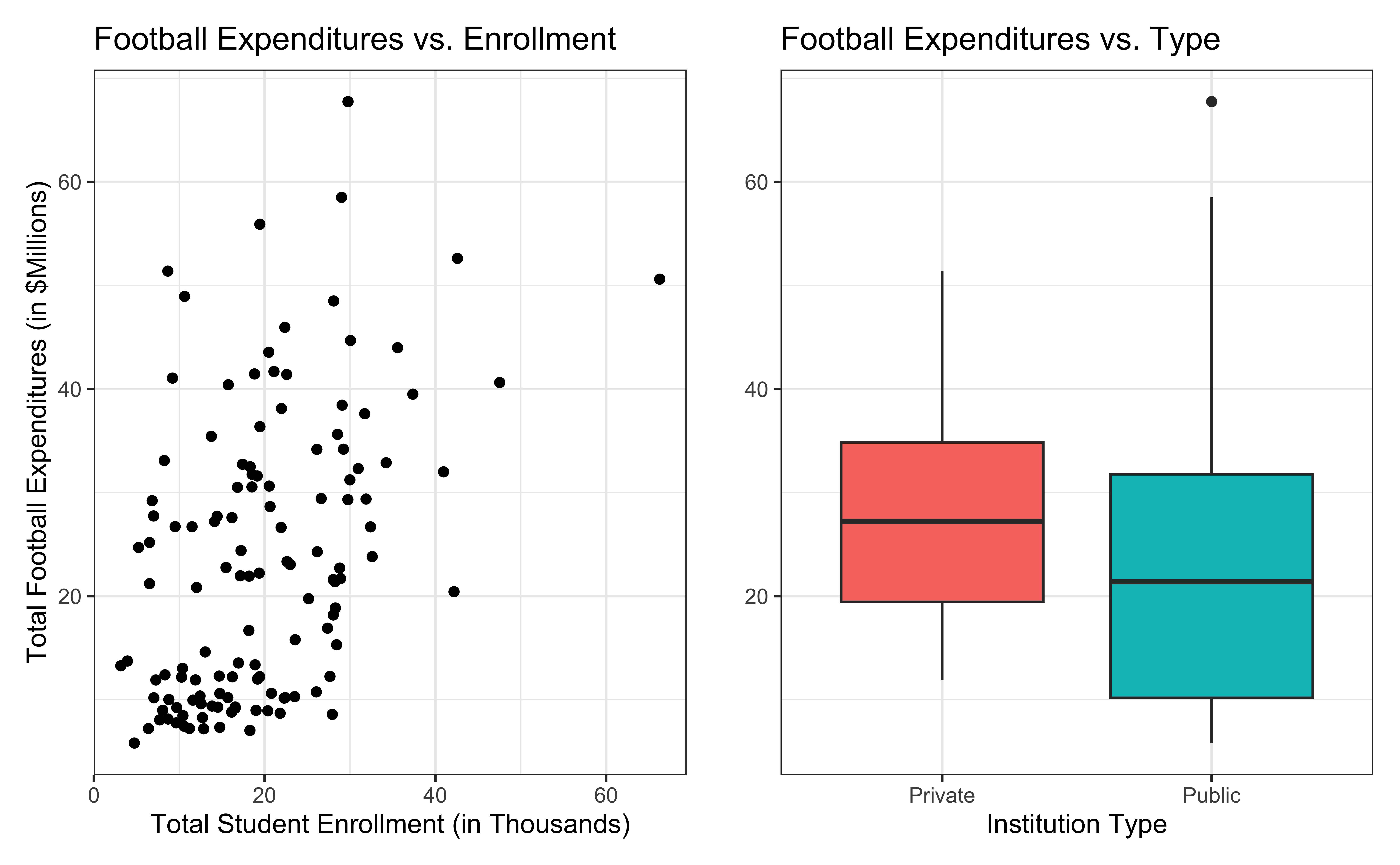
Data: NCAA Football expenditures
Today’s data come from Equity in Athletics Data Analysis and includes information about sports expenditures and revenues for colleges and universities in the United States. This data set was featured in a March 2022 Tidy Tuesday.
We will focus on the 2019 - 2020 season expenditures on football for institutions in the NCAA - Division 1 FBS. The following variables are used in this analysis:
total_exp_m: Total expenditures on football in the 2019 - 2020 academic year (in millions USD)enrollment_th: Total student enrollment in the 2019 - 2020 academic year (in thousands)type: institution type (Public or Private)
football <- read_csv("data/ncaa-football-exp.csv")Bivariate EDA
Regression model
exp_fit <- lm(total_exp_m ~ enrollment_th + type, data = football)
tidy(exp_fit) |>
kable(digits = 3)| term | estimate | std.error | statistic | p.value |
|---|---|---|---|---|
| (Intercept) | 19.332 | 2.984 | 6.478 | 0 |
| enrollment_th | 0.780 | 0.110 | 7.074 | 0 |
| typePublic | -13.226 | 3.153 | -4.195 | 0 |
0.780 is the exact relationship between football expenditure and enrollment for these 127 institutions in 2019-2020.
What if we want to say something about the relationship between these variables for all colleges and universities with football programs and across different years?
Statistical inference
Statistical inference provides methods and tools so we can use the single observed sample to make valid statements (inferences) about the population it comes from
For our inferences to be valid, the sample should be representative (ideally random) of the population we’re interested in
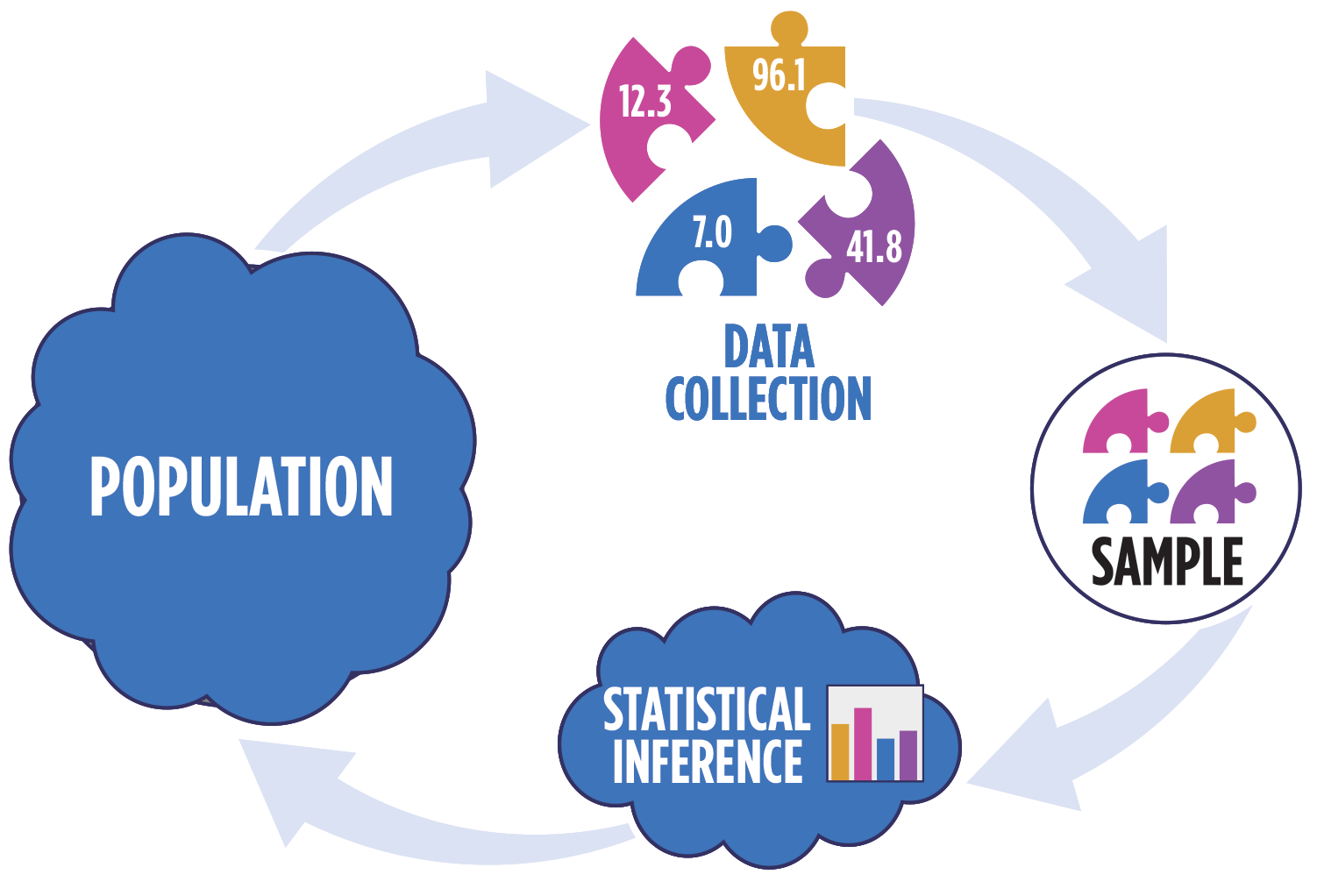
Inference framework
Our objective is to infer properties about a population using data from observational (or experimental) data collection
Pre data collection: Before collecting the data, the data are unknown and random. \(\hat{\boldsymbol{\beta}}\), which is a function of the data, is also unknown and random.
Post data collection: After collecting the data, \(\hat{\boldsymbol{\beta}}\) is fixed and known.
In all cases: The true population parameter, \(\boldsymbol{\beta}\) is fixed but unknown.
Question pre data collection: Is the probability distribution of \(\hat{\mathbf{\boldsymbol{\beta}}}\) a meaningful representation of the population? (We will slowly answer this question across the next few classes)
Linear regression model
\[\begin{aligned} \mathbf{Y} = \mathbf{X}\boldsymbol{\beta} + \boldsymbol{\epsilon}, \hspace{8mm} \boldsymbol{\epsilon} \sim N(\mathbf{0}, \sigma^2_{\epsilon}\mathbf{I}) \end{aligned} \]
such that the errors are independent and normally distributed.
. . .
- Independent: Knowing the error term for one observation doesn’t tell us about the error term for another observation
- Normally distributed: The distribution follows a particular mathematical model that is unimodal and symmetric
- \(E(\boldsymbol{\epsilon}) = \mathbf{0}\)
- \(Var(\boldsymbol{\epsilon}) = \sigma^2_{\epsilon}\mathbf{I}\)
Visualizing distribution of \(\mathbf{y}|\mathbf{X}\)
\[ \mathbf{y}|\mathbf{X} \sim N(\mathbf{X}\boldsymbol{\beta}, \sigma_\epsilon^2\mathbf{I}) \]
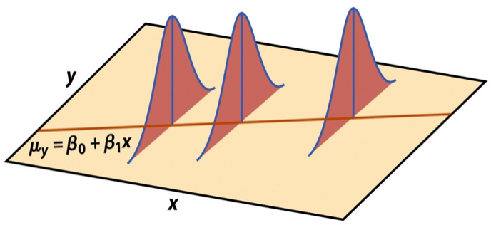
Last time we showed \(E(\mathbf{y}|\mathbf{X}) = \mathbf{X}\boldsymbol{\beta}\) and \(Var(\mathbf{y}|\mathbf{X}) = \sigma^2_{\epsilon}\mathbf{I}\)
Show \(\mathbf{y}\) is normally distributed
NoteLinear transformation of normal random variables
Suppose \(\mathbf{z}\) is a multivariate normal random variable. Then, \(\mathbf{Az} + \mathbf{b}\) is (multivariate) normal for \(\mathbf{A}\) a constant matrix and \(\mathbf{b}\) a constant vector.
Show that the distribution of \(\mathbf{y}|\mathbf{X}\) is normal.
Assumptions for regression
\[ \mathbf{y}|\mathbf{X} \sim N(\mathbf{X}\boldsymbol{\beta}, \sigma_\epsilon^2\mathbf{I}) \]
- Linearity: There is a linear relationship between the response and predictor variables.
- Equal variance: The variability about the least squares line is equal for all combinations of predictors.
- Normality: The distribution of the residuals is normal.
- Independence: The residuals are independent from one another.
Note
We will assume these hold for now and show how to check the assumptions after Exam 01.
Estimating \(\sigma^2_{\epsilon}\)
Once we fit the model, we can use the residuals to estimate \(\sigma_{\epsilon}^2\)
The estimated value \(\hat{\sigma}^2_{\epsilon}\) is needed for inference on the coefficients
\[ \hat{\sigma}^2_\epsilon = \frac{SSR}{n - p - 1} = \frac{\mathbf{e}^\mathsf{T}\mathbf{e}}{n-p-1} \]
. . .
- The regression standard error \(\hat{\sigma}_{\epsilon}\) is a measure of the average distance between the observations and regression line
\[ \hat{\sigma}_\epsilon = \sqrt{\frac{SSR}{n - p - 1}} = \hat{\sigma}_\epsilon = \sqrt{\frac{\mathbf{e}^\mathsf{T}\mathbf{e}}{n - p - 1}} \]
Inference for a single coefficient
Inference for \(\beta_j\)
We often want to conduct inference on individual model coefficients
Hypothesis test: Is there evidence of a linear relationship between the response and \(x_j\)? \((\beta_j \neq 0 ? )\)
Confidence interval: What is a plausible range of values \(\beta_j\) can take?
. . .
But first we need to understand the distribution of \(\hat{\beta}_j\)
Sampling distribution of \(\hat{\boldsymbol{\beta}}\)
A sampling distribution is the probability distribution of a statistic computed from many repeated random samples of size \(n\) drawn from a population.
The sampling distribution of \(\hat{\boldsymbol{\beta}}\) is the probability distribution of the estimated coefficients, formed by repeatedly taking sample of size \(n\) and fitting the regression model to compute \(\hat{\boldsymbol{\beta}}\)
\[ \hat{\boldsymbol{\beta}} \sim N(\boldsymbol{\beta}, \sigma^2_\epsilon(\mathbf{X}^\mathsf{T}\mathbf{X})^{-1}) \]
. . .
The estimated coefficients \(\hat{\boldsymbol{\beta}}\) are normally distributed with
\[ E(\hat{\boldsymbol{\beta}}) = \boldsymbol{\beta} \hspace{10mm} Var(\hat{\boldsymbol{\beta}}) = \sigma^2_{\epsilon}(\boldsymbol{X}^\mathsf{T}\boldsymbol{X})^{-1} \]
Expected value and variance of \(\boldsymbol{\hat{\beta}}\)
Show
\(E(\hat{\boldsymbol{\beta}}) = \boldsymbol{\beta}\)
\(Var(\hat{\boldsymbol{\beta}}) = \sigma^2_{\epsilon}(\boldsymbol{X}^\mathsf{T}\boldsymbol{X})^{-1}\)
Will show that \(\hat{\boldsymbol{\beta}}\) is normally distributed in the homework.
Sampling distribution of \(\hat{\beta}_j\)
\[ \hat{\boldsymbol{\beta}} \sim N(\boldsymbol{\beta}, \sigma^2_\epsilon(\mathbf{X}^\mathsf{T}\mathbf{X})^{-1}) \]
Let \(\mathbf{C} = (\mathbf{X}^\mathsf{T}\mathbf{X})^{-1}\). Then, for each coefficient \(\hat{\beta}_j\),
\(E(\hat{\beta}_j) = \boldsymbol{\beta}_j\), the \(j^{th}\) element of \(\boldsymbol{\beta}\)
\(Var(\hat{\beta}_j) = \sigma^2_{\epsilon}C_{jj}\), where \(C_{jj}\) is the \(j^{th}\) diagonal element
\(Cov(\hat{\beta}_i, \hat{\beta}_j) = \sigma^2_{\epsilon}C_{ij}\)
Application exercise
Questions
Recap
- Derived the distribution of the coefficients \(\hat{\boldsymbol{\beta}}\)
Next class
- Hypothesis tests and confidence intervals for a coefficient \(\beta_j\)
- Complete Lecture 09 prepare